Knowledge distillation

Knowledge distillation has become a cornerstone technique for training capable smaller language models. The recipe seems straightforward: generate high-quality responses from capable teacher models, then train a student model on these examples. Unfortunately, student models learning from knowledge distilled from multiple capable teachers don't necessarily perform well, mixing responses from multiple teacher models often produces worse results than using a single teacher*, even when each individual teacher is highly capable.

This phenomenon, sometimes called the "knowledge conflict", "style inconsistency", or "teacher heterogeneity" issue, has been observed repeatedly and is open knowledge in frontier labs, but remains underexplored in the literature.

The Empirical Observation

Recent work has documented the multi-teacher distillation problem directly. Jin et al. (2026) found that "contrary to expectation that enlarging the teacher LLM ensemble would enhance the capabilities of student models, the distillation performance actually declines as the number of teacher models further increases". This decline persists even when each additional teacher is individually capable.

The PerSyn paper similarly observes that "stronger models are not always optimal teachers for small student models, since their outputs may be overly complex and shift away from the students' distribution". Simply mixing synthetic data from multiple teachers leads to suboptimal performance.

But why? Each teacher produces correct, high-quality responses. Shouldn't more diverse training data help?

The Distributional Perspective

To understand what's happening, we need to think about what the student model is actually learning during supervised fine-tuning (SFT).

Single Teacher: A Coherent Target

When training on data from a single teacher, the student learns to approximate that teacher's output distribution:

The teacher's distribution, while complex, is coherent—it reflects a single model's learned patterns for formatting, hedging, explanation structure, and stylistic choices. The student has a clear target to fit.

Figure 1: With a single teacher, the student learns to approximate a unimodal distribution. The optimization objective is clear.

Multiple Teachers: Superimposed Distributions

When training on data from multiple teachers, the student sees a mixture:

If the teachers have different stylistic patterns—different ways of starting explanations, different hedging phrases, different levels of verbosity—then the training distribution is multimodal. The student must fit multiple overlapping but distinct distributions simultaneously.

Figure 2: With multiple teachers, the training distribution becomes multimodal. Each teacher contributes a distinct mode.

What Does the Student Actually Learn?

SFT with cross-entropy loss on multimodal data tends to produce an interpolated distribution.

When the student model lacks the capacity or signal to separate the modes, it learns something like the average:

This interpolated distribution may not correspond to any coherent generation behavior. It places probability mass in regions between the modes—outputs that neither teacher would produce.

Figure 3: The student learns an interpolated distribution that doesn't match any individual teacher. The resulting outputs may be incoherent—blending styles in ways no real model would.

Concrete Example

Consider how different models explain a mathematical concept:

Teacher A (Concise):

"The derivative of x² is 2x. This follows from the power rule: d/dx[xⁿ] = nxⁿ⁻¹."

Teacher B (Verbose):

"Let me walk you through finding the derivative of x². We'll use the power rule, which states that for any function f(x) = xⁿ, the derivative is f'(x) = nxⁿ⁻¹. Applying this with n=2, we get d/dx[x²] = 2x²⁻¹ = 2x. This is our final answer."

A student trained on both might produce:

Student (Interpolated):

"Let me explain. The derivative of x² is 2x. We use the power rule."

This response is neither the clean conciseness of Teacher A nor the thorough walkthrough of Teacher B. It's an awkward middle ground that represents neither distribution well.

What to do instead?

While many different distillation methods have been presented in the literature for multi-teacher knowledge distillation, many involving clever weighting and estimation of teacher models and their "expertise", the leading open-source model developers—DeepSeek, Qwen, Kimi, and others—have converged on a pattern that sidesteps this problem: specialist models derived from the same base model.

The Specialist Distillation Pattern

The general recipe, as observed in multiple model releases:

1. Train base model on large-scale pretraining data
2. Create specialists by fine-tuning the base on domain-specific data (math, coding, reasoning, etc.)
3. Generate training data from specialists on prompts in their respective domains
4. Train general model by distilling from all specialists back to the base

Crucially, all specialists share the same base model. This means they share:

• The same vocabulary and tokenization
• Similar underlying representations
• Consistent formatting tendencies inherited from base training
• Related but not identical output distributions

Figure 4: Specialists from the same base model have distributions that are shifted versions of each other, not entirely different distributions. The interpolation problem is greatly reduced.

Why Same-Family Specialists Work

When specialists derive from the same base:

1. Distributional similarity: Their output distributions are perturbations of a shared prior, not arbitrary distributions
2. Style inheritance: Domain-specific fine-tuning changes what the model knows more than how it expresses things
3. Bounded divergence: The amount of post-training data for specialization is small relative to pretraining, limiting distributional drift
   • This also gives insight to the scale of data that is needed to overcome the knowledge conflict problem when distilling from multiple teachers, which is likely bigger than that of typical SFT data size.

The student learning from same-family specialists isn't trying to fit arbitrarily different distributions—it's fitting distributions that are already close in the space of possible outputs.

The Motivation: Why Not Just Mix All the Data?

A natural question arises: why go through the trouble of training separate specialists and then distilling? Why not simply combine all the domain-specific training data and train a single model on the mixture from the start?

The two-stage specialist approach offers several advantages:

1. Avoiding catastrophic forgetting during training: When training a single model on mixed data, aggressive optimization on one domain can degrade performance on others. Specialists can be pushed harder on their specific domain without this concern.

2. Flexible data ratios at distillation time: With specialists, you control the mixture ratio when generating synthetic data, not when training. This is a much easier hyperparameter to tune—you can regenerate data at different ratios without retraining models.

3. Domain-specific training techniques: Different domains may benefit from different training approaches (curricula, loss functions, data augmentation). Specialists allow domain-specific optimization that would conflict if applied simultaneously.

4. Independent quality control: Each specialist can be evaluated and iterated on independently. If your math specialist underperforms, you fix it without touching the code specialist.

5. Selective distillation: The distillation process can cherry-pick the best outputs from each specialist via rejection sampling. Direct data mixing doesn't offer this quality filtering opportunity.

6. Compute efficiency for iteration: Updating one capability requires retraining only that specialist and regenerating its contribution to the distillation data, not retraining the entire model.

7. Organizational simplicity: Each specailist model can have a separate team associated with it in the organization, simplifying human communication overhead.

The key insight is that the distributional consistency comes from the shared base model, not from training on mixed data. Specialists diverge in what they know, but retain similar patterns for how they express it—making their outputs compatible for distillation even though they were trained separately.

Evidence from Practice: The DeepSeek-R1 Example

The DeepSeek-R1 paper provides a particularly clear example of this pattern applied to reasoning. Their pipeline:

1. DeepSeek-R1-Zero: Apply large-scale RL directly to the base model (DeepSeek-V3-Base) without SFT. This produces a specialist reasoning model with emergent chain-of-thought behaviors—but also issues like poor readability and language mixing.

2. Rejection sampling: Generate reasoning solutions from R1-Zero, filter for correctness.

3. Combined SFT: Train the final R1 model on a mixture of:

   • Reasoning data from R1-Zero (the reasoning specialist)
   • Non-reasoning data from DeepSeek-V3's existing SFT data (writing, factual QA, etc.)

Critically, both the reasoning specialist (R1-Zero) and the non-reasoning data source (V3) derive from the same base model. The paper explicitly notes that "we create new SFT data through rejection sampling on the RL checkpoint, combined with supervised data from DeepSeek-V3 in domains such as writing, factual QA, and self-cognition."

• the reasoning patterns come from one specialist (R1-Zero),
• general capabilities from another (V3's post-training)

Both share the V3-Base foundation. The result maintains coherent outputs while gaining specialized reasoning abilities.

• Qwen follows a similar iterative improvement loop with domain specialists
• The general model benefits from domain transfer while maintaining coherent outputs because all teachers are consistent stylistically.

Connection to Reasoning Mode Training

The rise of "thinking" models—those with explicit reasoning traces enclosed in <think> tags—introduces a new dimension to this problem.

Reasoning as a Separate Distribution

Models like DeepSeek-R1, o1, and Claude's extended thinking learn two distinct output modes:

1. Direct mode: Standard assistant responses (System 1)
2. Thinking mode: Extended reasoning traces followed by answers (System 2)

These modes have different distributional characteristics. Thinking mode features:

• Longer outputs with self-correction
• Exploratory hypothesizing
• Step-by-step decomposition
• Different transitional, introspective phrases ("Let me reconsider...", "Wait, that's not right...")

Is This Multi-Teacher Distillation?

One might ask: if we train a model to have both thinking and non-thinking modes, aren't we effectively training on two different distributions?

Yes, but with a crucial difference: the mode is explicitly marked.

<no_think_token> → Distribution A (direct responses)
<think_token> → Distribution B (reasoning traces)

The <think> token acts as an explicit conditioning signal. The model doesn't need to infer which distribution applies—it's directly specified. This converts the problem from:

• Implicit mixture (bad): Learn to somehow fit both distributions without knowing which is which
• Conditional distributions (tractable): Learn $P(\text{response}\mid \text{prompt},\text{mode}=\text{direct})$ and $P(\text{response}\mid \text{prompt},\text{mode}=\text{thinking})$ separately

Figure 5: With explicit mode tokens, the model learns conditional distributions rather than a confused mixture. The token boundary provides clear separation.

The Bimodality Hypothesis

This suggests a hypothesis: explicit mode separation via special tokens can allow different "teachers" for different modes.

Specifically:

• Thinking mode could use reasoning traces from a strong reasoning model
• Direct mode could use responses from a stylistically preferred model
• The mode tokens prevent cross-contamination

The student learns:

• Inside <think>: Reasoning patterns from the reasoning model
• After </think>: Answer style from the preferred model

This is a form of multi-teacher distillation, but the explicit structure potentially makes it tractable. However, this doesn't mean naive application will work in practice. Suppose the model successfully learns to output reasoning process in thie <think></think> block and direct answer outside. The distribution differences between these two modes can be so drastic such that the direct answer doesn't follow from the reasoning tokens. This is not unreasonable -- there's nothing forcing the reasoning logic to "transfer" to the direct answer. Therefore reasoning models trained this way may result in having correct "thoughts" leading to an incorrect answer.

Implications and Open Questions

For Practitioners

1. Prefer single teachers when possible. The simplicity pays off in coherent outputs.

2. If mixing teachers, measure style divergence first. For example, train a classifier to predict which teacher generated a response. High accuracy = high divergence = likely problems. Distilling from the "best math model" and the "best creative writing model" may not lead to the "best math + writing" model.

3. Same-family specialists are safer than arbitrary model combinations. If you must use multiple teachers, prefer those from the same base model.

4. Explicit mode separation helps. If you need different capabilities (reasoning vs. direct), consider explicit mode tokens rather than implicit mixing. There are methods that can improve non-explicit mixed-mode performance though.

Open Research Questions

1. How much style divergence is too much? Is there a threshold below which multi-teacher mixing is safe?

2. Can rewriting normalize styles effectively? Having one model rewrite another's outputs might help, but at what cost to content fidelity?

3. Do larger students handle multimodality better? Perhaps sufficient model capacity can maintain separate modes implicitly.

4. What's the role of data scale? With enough data, does the distributional mismatch problem diminish?

Conclusion

The empirical observation that multi-teacher distillation often underperforms has a natural explanation: training on multimodal data from heterogeneous teachers leads to interpolated distributions that don't correspond to coherent generation behavior. The student learns to produce outputs that fall between the modes—satisfying neither teacher's distribution well.

The research community has responded with practical solutions: using specialists from the same model family, which constrains distributional divergence, and employing explicit mode tokens, which convert implicit mixtures into tractable conditional distributions.

As models become more capable and distillation pipelines more complex, understanding these distributional dynamics becomes increasingly important. Style consistency isn't just an aesthetic preference—it's a fundamental property that determines whether a student can learn coherently from its teachers.

DeepSeekMath-v2 came out on Thanksgiving without much fanfare but has now become the only open weight model to achieve IMO-gold performance with natural language informal proofs, after Gemini and GPT5. The technical reported is a packed with technical details, much of which isn't entirely surprising as the entire LLM field has converged toward a similar direction in terms of how to achieve iterative improvements in a domain like informal math proofs.

Key ideas

How to verify?

In the past year, RL with verifiable reward (RLVR) has made a lot of stride, especially in math and coding domains. After GPT-4o, Deepseek-R1 paper really popularized this approach (history repeating itself with DeepseekMath-v2 now). However, for something not easily verifiable like math proofs, how to craft a reward function that provides a training signal?

In other words, how to verify math proofs better to provide a training signal to improve proof generation?

Taking inspiration from human proof verification, we notice that:

• Issues can be identified in a proof even without reference solution. Whether this is by pattern matching a familiar subproblem and noticing a wrong solution, or by noticing inconsistent logical statement even if one cannot verify how the predicates and conclusion of a logical statement were derived.
• A proof is more likely to be valid when no issues can be identified after "thinking for a long time by a lot of different people". This is similar to the scientific peer review process. In LLM speak, this means that a proof is more valid if "after scaled verification efforts no issues can be identified".

So the answer to "how to verify better" is then "scaling verification compute".

What's "scaling verification compute"?

This is in line with scaling test time compute. In the case of DeepseekMath-V2, this is parallel inference with majority-voting, which does the following:

Given a proof, how do we verify its correctness better?

• Give the proof to the verifier model, ask it to evaluate the proof according to some rules.
• Do this in parallel for $N$ times.
• If most of the generated verifications think there's no problem, then proof is probably good.
• If at least $k$ of the generated verifications think that there's some kind of problem, then proof probably has a problem.
• If no group of $k$ verifications agree on a correctness score, then the verifier is too unsure of the proof quality -- this means the verifier is not smart enough to check the work of that proof. We can discard this specific proof rollout.

How to improve proof-generation ability?

The verifier with scaled compute can now provide a reward signal to improve proof generation in an RL setting. This reduces to the classic RLVR-by-GRPO:

1. For each problem $x$, generate $P$ proofs from the model.
2. For each proof $y_i$, do scaled verification (so $N$ times per proof), and get the resulting proof's score $s_i$ from majority voting -- this results in a set of {$y_i$, $s_i$} for each problem.
3. Combine each $s_i$ with other rubrics to get a final reward score $r_i$ for $y_i$.
4. Do backprop with the reward score.

The reward score for proof-generation is set to be $R_Y=s$.

At the end of a round of RL, we can additionally do SFT for each problem $x$ with proofs verified to be correct. This will distill and improve the model's proof generation capability further.

Maintaining generation-verification gap

An assumption that is implied in the above approach is that verification is easier than generation, this is known as the "generation-verification gap". This has the same intuition as P != NP -- the widely believed but unproven statement that problems whose solutions are easy to verify (P) are not necessarily easy to solve (NP).

Scaling verification compute to verify generated proofs by the LLM can work IF there exists a gap between the proof generator and the proof verifier. But as RL improves the generator, this gap shrinks and performance eventually saturates, and the rate of this saturation has been shown to correlate to the models' pretraining flops.

Therefore to continuously improve generator abilities, the verifier capability needs to improve as well -- in other words, the generation-verification gap needs to be maintained.

This means the verifier needs to be continously trained somehow, with dataset of {proof, proof score}. This was provided exactly during the proof-generation rollout process!

With this data, RLVR-by-GRPO for verification generation can proceed similarly. The obvious reward term is:

where $s_i^{\prime }$ is the score given to the proof by the i-th verification rollout, and $s_i$ is the "ground-truth" proof score from the proof generation step. We want each verification rollout to match the consensus score for a proof.

Additionally, there's format reward $R_{format}$ to reward certain verification format.

Prevent verifier hallucination with meta-verification

With only $R_{score}$ and $R_{format}$, the verifier can assign a correct score to the proof while still hallucinating non-existent issues. To prevent this, verification of proof verification reasoning can be introduced -- metaverification.

The underlying idea here is again the generation-verification gap -- it's easier to verify the verifications than generating the verifications. Here, for each verification, a metaverification is generated to find issues in the verification analysis with an accompanying verification quality score $ms$. This score $R_{meta}$ is then added to the verifier training reward term:

In the end, the verifier can both verify proofs, and verify those verifications.

Meta-verification as an additional scaling axis?

All problems in computer science can be solved by another level of indirection [...] except for the problem of too many levels of indirection

The above is a a piece of engineering common wisdom that's also used often as a meme/joke. It's often applied in situations where the solution is to apply an extra layer of abstraction (e.g. virtual memory, file descriptors, DNS, abstract classes/interfaces, containers, etc). The use of meta-verification reminded me of this.

Metaverification here takes the advantage of the verification-generation gap. It's unclear how fast the metaverification-verification gap reduces compared to the verification-generator gap, and how that relative convergence varies for problem domains. Perhaps multiple layers of metaverifications can become a trick to prevent verifier performance saturation?

Alternatively, we can think of meta-verification as introducing additional layer of model "feedback-loop" to amplify its abilities.

Forcing self-verification during proof generation

The authors points out that

when a proof generator fails to produce a completely correct proof in one shot [...] iterative verification and refinement can improve results. This involves analyzing the proof with an external verifier and prompting the generator to address identified issues.

But in practice:

while the generator can refine proofs based on external feedback, it fails to evaluate its own work with the same rigor as the dedicated verifier

What this means:

• Scenario: The model generates a flawed proof.
• Standard Behavior: The model concludes "Therefore, the answer is X" and internally assigns it a high confidence.
• The Consequence: Because the model thinks it is right, it stops. It never triggers a refinement loop because it doesn't believe there is anything to fix.

While the model could fix the error if an external teacher pointed it out, it fails to find the error itself.

The authors then refined the proof-generation prompt and updated the reward function to force the model to rigorously "identify and resolve as many issues as possible before finalizing the response" (i.e. a type of test-time compute scaling by increasing reasoning chain length).

This is done by:

• In addition to the proof $Y$ generated, the prompt also asks the model to generate a self-analysis $Z$ of the proof $Y$ according to the same rubric given to the verifier.
• The proof $Y$ receives score $R_Y=s^{\prime }$, and the self-analysis $Z$ receives metaverification score $R_{meta}(Z)=ms$.

The reward function then becomes:

So the verifier will check the proof generated, and the associated self-analysis. This then incentives the model to think harder and not be lazy.

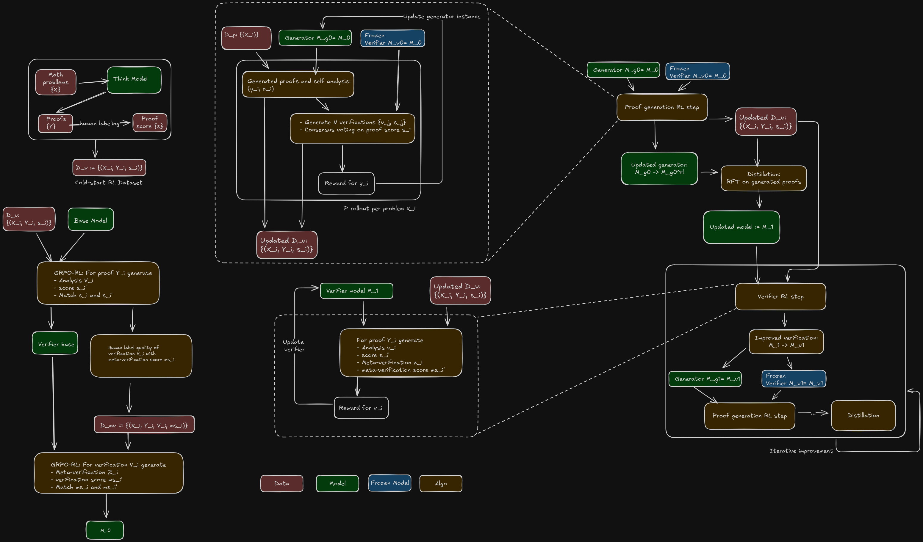
Iterative improvement

Now all pieces are in place to do continuous iterative improvement. Note that even though we talk about "verifier" and "generator", they are in fact the checkpoints of the same model. Let $M_0$ be the model at the start of the process.

In iteration 0, we have the following steps:

1. Initalize proof verifier $M_{v0}$ from $M_0$ and freeze it.
2. Initialize proof generator $M_{g0}$ from $M_0$. Use it for proof-generation RLVR with $M$ rollouts:
   • for each problem $x$, generate $P$ proofs.
     • for each proof $y_i$ and associated self-analysis $z_i$, generate $N$ verifications
       • Conduct consensus voting among the $N$ verifications to either assign a score $s_i$ to each proof for reward calculation (and associated metaverification score $m{s}_i$ for $z_i$), or discard that proof if no consensus.
   • backpropagate all the reward signals on the generated proofs and self-analyses.
   • At end of each iteration, we also save $D_V=(X,Y,s)$ -- triplets of problem, proof, and proof score for verifier training.
   • After this process, $M_{g0}$ updated to $M_{g0}^{rl}$.
3. Do distillation via SFT on $M_{g0}^{rl}$ with correct proof rollouts, i.e. subset of $D$ where $s=1$, this gives us $M_1$.

In iteration 1 and on, we have:

1. Do verification-generation rollout with $M$ rollouts on $M_i$.
   • for each proof $y$, generate $N$ verifications and metaverifications
     • for each verification $v_i$, metaverification $m{v}_i$, and associated proof score $s_i^{\prime }$, calculate reward score $R_V$.
   • At end of this process, $M_i$ is updated to $M_{vi}$.
2. [Not explicitly stated in the paper]: The metaverification ability can also be improved via RL here. For each $(y_i,s_i)$ from the previous round, generate metaverifications $z_i,m{s}_i$ and perform consensus voting to obtain "ground-truth" metascore $z_i$. The RL process reward metaverification rollout metascore $z_i^{\prime }$ to match $z_i$.
3. Freeze $M_{vi}$.
4. Initialize proof generator $M_{gi}$ from $M_{vi}$. Do proof-generation RLVR with $M$ rollouts. After this step, $M_{gi}$ becomes $M_{gi}^{rl}$.
5. Do SFT on $M_{gi}^{rl}$ with correct proof rollouts, resulting in $M_{i+1}$.

Important details

Model initialization and cold-start

Before the iterative improvement can begin, SFT is needd to improve the baseline generation and verification performance -- otherwise a lot of inference compute would be wasted to derive easy facts. Fortunately the base model DeepSeek-V3.2-Exp-Base already has reasonable math capabilities.

Cold-start verifier RL dataset

To start verifier RL training, a set of hard problems, proofs and estimates of proof quality is needed.

1. Curate $D_p$ by crawling hard math problems (e.g. IMO, USAMO, CMO, etc) that require proofs.
2. Generate candidate proofs using Deepseek-V3.2-Exp-Thinking -- a capable thinking model. The prompt used iterative-refinement to ask the model to improve its proofs to improve the proof quality.
3. Sample from this pool of generated proofs and have humans annotate the proof quality.

This process yields the initial RL-dataset $D_v=(X_i,Y_i,s_i)$ -- triplets of problem, proof, and annotated proof score.

Cold-start metaverifier RL dataset

Similarly, annotations are needed to initiate RL training for the metaverifier.

1. The verifier generates proof verification $V_i$ ($s_i$ is part of this) for proof $Y_i$.
2. Human experts annotate $V_i$ according to some rubric to arrive at a verification score, $m{s}_i$.
3. The resulting dataset $D_{mv}=(X_i,Y_i,V_i,m{s}_i)$ is used to train the metaverifier (same as the verifier) to produce a summary of issues found in each verification $V_i$ and produce a verification score $m{s}_i^{\prime }$ to match $m{s}_i$.

Inference: Sequential refinement with verification

Iterative self-refinement is a test-time inference scaling idea introduced around 2023 (self-refine, ReAct). This technique is similar to how humans try to iteratively refine a solution:

1. Model generates an answer
2. Prompts the model verifies and spots mistakes in the answer and proposes solution
3. Prompt the model to generate an answer again, taking into account of its own analysis in (2).
4. Iterate 2-3 multiple times

Notice with this method, while the quality of the proof improves with additional iterations, its ultimately limited by the verifier's ability!

The process of iterative self-refinement can additionally be parallelized (i.e. having multiple people thinking about the same problem repeatedly). The final answer can then be determined by committee among the different threads' answers (i.e. via majority voting, another synthesizer model decided based on their results, etc)

High-Compute Search (Population-Based Refinement)

For the most challenging problems where standard sequential refinement fails, the paper proposes a "High-Compute Search" that scales both generation (breadth) and verification (depth). Instead of refining a single thread, this method evolves a population of proofs.

1. Initialization: A pool of candidate proofs is initialized (e.g., 64 samples).
2. Mass Verification: For each proof in the pool, the model generates 64 independent verification analyses. This statistical volume helps identify subtle issues that a single verification pass might miss.
3. Selection & Pairing: The system selects the 64 highest-scoring proofs based on their average verification scores. Each selected proof is paired with 8 verification analyses, specifically prioritizing those that identified issues (scores of 0 or 0.5).
4. Evolution: Each <proof, analysis> pair is used to generate a new, refined proof, which updates the candidate pool.
5. Termination: The process repeats for up to 16 iterations or until a proof passes all 64 verification attempts (unanimous consensus), indicating extremely high confidence in correctness.

This method is used to eventually take IMO 2025 and Putnam 2024 achieving incredible scores.

Step 3 seems rather strange -- pairing high-scoring proofs with randomly sampled verification you are bound to end up with <proof, analysis> pairs where the analysis is simply irrelevant to the proof. I wonder how often this actually generates a better proof than the existing pool, in other words, how compute efficient this is.

Why this works and what next?

The success of AlphaGo and AlphaZero were major inspirations for a lot of the iterative improvement approaches. But the approaches there are hard to translate into iterative improvement in LLMs, as previously explained in DeepSeek-R1:

we explored using Monte Carlo Tree Search (MCTS) to enhance test-time compute scalability. This approach involves breaking answers into smaller parts to allow the model to explore the solution space systematically. To facilitate this, we prompt the model to generate multiple tags that correspond to specific reasoning steps necessary for the search. For training, we first use collected prompts to find answers via MCTS guided by a pre-trained value model. Subsequently, we use the resulting question-answer pairs to train both the actor model and the value model, iteratively refining the process.

However, this approach encounters several challenges when scaling up the training. First,unlike chess, where the search space is relatively well-defined, token generation presents an exponentially larger search space [...] Second, the value model directly influences the quality of generation since it guides each step of the search process. Training a fine-grained value model is inherently difficult, which makes it challenging for the model to iteratively improve.

In conclusion, while MCTS can improve performance during inference when paired with a pre-trained value model, iteratively boosting model performance through self-search remains a significant challenge.

The MCTS in AlphaGo/Zero was hard to replicate because:

1. The LLM token space is hard to define as a search problem useful for MCTS.
2. The value function used to guide the search is hard to define.

GRPO-style RL solves (1) by replacing tree search with parallel sampling (exploration), and applying the same to verification solves (2) by using verifiers as the reward model. Now, iterative improvement is possible.

The core mechanism in both systems is using compute-heavy search to generate high-quality data, then distilling that data back into the model to improve its "instinctive" capabilities.

It's obvious that iterative improvement for a verifiable domain like Go should work. The intuition behind why it should work for a hard-to-verify domain like math proofs is less so, and I understand it as the following:

1. Consensus Voting as Noise Reduction Individual model outputs are noisy samples from a probability distribution. By sampling $N$ verifications and taking a majority vote (especially when cross-checked by a Meta-Verifier), we effectively reduce the variance.
   - The "Consensus Label" is a far higher-fidelity approximation of the "Ground Truth" than any single model inference.
   - Training on this consensus effectively "denoises" the model's understanding of what constitutes a valid proof.
   - Known in the field as "self-consistency"
2. Manifold Expansion via Search and Distillation We can view the "space of correct mathematical proofs" as a low-dimensional manifold within the high-dimensional space of all possible text.
   • RL/Search (The Reach): Standard generation samples near the center of the model's current manifold. Iterative Refinement (Test-Time compute scaling or multiple rounds of RL) allows the model to traverse off its comfortable manifold, stepping through error-correction to find a distant solution point (a hard proof) that it could not generate zero-shot.
   • Distillation (The Pull): By performing SFT/RFT on these distant solution points, we pull the model's base distribution (manifold) towards these new regions
   • The Result: The "center" of the manifold shifts. Problems that previously required expensive search (edges of the manifold) are now near the center (zero-shot solvable).
3. The Difficulty Ceiling As the model improves, the manifold covers the entire training distribution. The limiting factor becomes the difficulty of the problems. If the model can solve everything in the dataset zero-shot, the gradient for improvement vanishes. To exceed the best human capability, the system eventually needs a mechanism to generate novel, harder problems (synthetic data generation) or prove open conjectures where the ground truth is unknown, relying entirely on its self-verification rigor to guide the search into uncharted mathematical territory -- this is likely needed for "superintelligence".

This intuition is well-observed in human learning: we improve the fastest when we are attempting tasks that are SLIGHTLY out-of-reach. In fact, the "search" and "verifier" in LLM iterative improvement are analogous to "information" in the Challenge Point Framework for optimal learning difficulty.

One of the most well-known understanding in the field of LLM currently is that “pretraining is where the model learns knowledge”, SFT and RL then elicit/shapren this knowledge to make them useful. I'm not entirely sure what first popularized this (could just be due to academic diffusion), but the first well-known paper of might've been the LIMA paper (May 2023), which suggests that:

Taken together, these results strongly suggest that almost all knowledge in large language models is learned during pretraining, and only limited instruction tuning data is necessary to teach models to produce high quality output.

This introduced the notion that a model’s capability is upper bound by the quality of the pretraining data, and that the better the pretraining is, the more benefits SFT will be. A corollary of this is that focusing on SFT too much can degrade general model capabilities in other tasks (e.g. reasoning and math).

A later paper, Revisiting the superficial alignment hypothesis (Sept 2024) dispute this:

We re-examine these claims by empirically studying the scaling behavior of post-training with increasing finetuning examples [...] Through experiments with the Llama-3, Mistral, and Llama-2 model families of multiple sizes, we observe that, similar to the pre-training scaling laws, post-training task performance scales as a power law against the number of finetuning examples. This power law relationship holds across a broad array of capabilities, including mathematical reasoning, coding, instruction following, and multihop-reasoning. In addition, for tasks like math and multihop reasoning, we observe that a handful of examples merely align the model stylistically but do not saturate performance on the benchmarks. Model performance is instead correlated with its reasoning ability and it improves significantly with more examples. We also observe that language models are not necessarily limited to using knowledge learned during pre-training. With appropriate post-training, a model’s ability to integrate new knowledge greatly improves on downstream tasks like multihop question-answering.

This paper then provides evidence against the “knowledge base is formed only in pretraining” understanding. Traditionally (e.g. 2022), LLM training consists of pretraining, midtraining (on data of specialized domain e.g. STEM), instruction-tuning/SFT, and RL. Subsequently it’s becoming clear that focusing on SFT alone can provide has outsized returns:

• Models benefit from learning from QA data, if it’s high quality and have diverse prompt format
• The resulting model also learns how to act as an assistant (style alignment)

This style of training allows the introduction of additional tricks such as Rephrasing. First widely introduced in Llama3 and now used in more models like Kimi, to create more synthetic training data from existing data. This technique rephrases text in different ways, and creates question-answer pairs from this text in different styles. This can be thought of as a form of data augmentation, encouraging model generalization.

What about Style-locking?

In vanilla instruction-tuning, the model is shown the prompt, and generates the response tokens with the objective of matching the response token distribution with that of the reference response, while MASKING the loss of the prompt tokens. In other words, in instruction-tuning, the response generation is always conditioned on the prompt. A potential concern might be that this can degrade the model’s generative ability and learn to only output in question-answer format, such that if prompted something non-standard like “1, 2, 3, 4,...” it would shit the bed.

Yet another trick and observation regarding this is found in Instruction following without instruction tuning (Sept, 2024), associated blogpost. It found that:

Adaptations like training only on poetry, or only on responses without corresponding instructions, yield models that follow instructions. We call this implicit instruction tuning.

Language models are, in some sense, just really prone to following general instructions, even when our adaptation strategies don’t teach the behavior directly. We call this implicit instruction tuning.

In other words, training only on RESPONSES of QA-pairs would elicit proper instruction-following, which removes this concern of rigid style and degraded generative ability. This phenomenon is very interesting, as it’s not an obvious result. One potential hypothesis is that being able to predict the responses means the model would have to understand the context around them (i.e. “I’m likely reading a response to a question”).

So now, SFT can be simplified to: train on diverse and high-quality RESPONSES to QA pairs. Note here “quality” is essentially “long chain-of-thought” style text.

It’s great to see the field simplifying and focusing on what matters the most. A recent paper from Nvidia (Sep, 2025) investigates the interaction of data and phase of training, specifically,

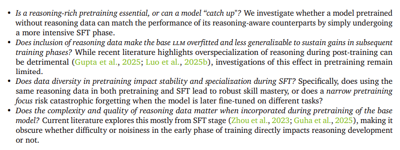
Is adding reasoning data earlier during pre-training any better than introducing it during post-training, when the token counts are controlled? Could earlier inclusion risk overfitting and harm generalization, or instead establish durable foundations that later fine-tuning cannot recover?

This paper investigates the following specific hypothesis:

with conclusions

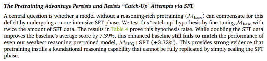
and most importantly refute the SFT-reasoning catchup hypothesis at the end:

This is unfortunate, as pretraining is often the most costly part of LLM training.

Note that the Nvidia paper still concludes that

SFT is a phase of targeted refinement, not broad data absorption

this is in direct conflict with the “Revisiting the superficial alignment hypothesis” paper, which concludes from new-fact learning experiments that:

if the model is first post-trained to do reasoning, it gets better at absorbing new information and using it in multihop reasoning tasks.

In terms of experiment setup, the Nvidia paper’s conclusion about SFT being targeted refinement seems weaker, as its conclusion derives from the observation that naively doubling SFT dataset with mixed quality data does not improve model performance compared to adding small amount of high quality data.

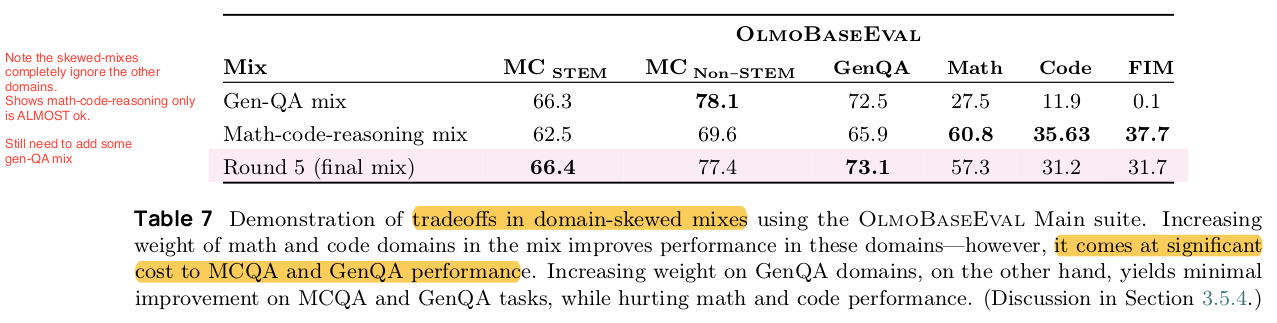
In a similar vein, the recently released OLMO3 showed a cool ablation study comparing the effects of including reasoning/stem data vs not into midtraining stage (total 100B tokens) and showed asymmetrical benefits of different data types to downstream model capabilities.

In conclusion, the basic intuition is the same:

• Pretraining data needs to be diverse and have a high scale. Having reasoning data is useful and raises the upper bound.
• SFT data needs to focus on high quality, and indeed, quality > quantity here.

The details are simplifying:

• Training on simply the responses of high quality SFT/Instruction-tuning data is enough to both elicit proper instruction tuning, model capability, and instill reasoning abilities, without degrading other general abilities significantly (e.g. creative-writing).

But perhaps even having a distinction between pretraining, mid-training, and SFT-post-training is an unecessary division. The only meaningful difference is just the learning rate. Perhaps eventually, the boundaries here will be blurred even more and dynamic learning-rate tuning will become the norm.

What underlying principle hypothesis can be used to explain these observations? Perhaps a good title for a review paper could be "The unreasonable effectivness of reasoning data".

• Models learn semantics, language distribution, and a naive world model from pretraining. Here scale and diversity is important because we want to sample the language distribution as widely as possible.
• Big problems with language models are hallucination and reliable long horizon reasoning – these abilities have lower entropy and requires higher generalization
  • To combat this problem, we need lots of high quality (e.g. long COT, multi-hop, coherent reasoning) data.
  • Yet the process is robust enough such that improvement in reasoning abilities doesn’t necessarily compromise higher entropy tasks performance significantly.

I suspect that language structure likely contributes to the unreasonable effectiveness of reasoning data!

But another explanation could simply be...almost all useful tasks and evals for LLM depend on having robust reasoning and applying them to construction and deductions from assumptions and given info, so it only makes sense that having more high-quality reasoning data in all stages of training benefits model performance 🤷‍♂️

GRPO-style RL-post training is great, as Deepseek-R1 first showed. But there are some big obstacles, mainly due to data efficiency:

• As the model gets smarter, we need more and more difficult problems – this now requires expert human labeling. How to do this with synthetic data?
• Plain RL with GRPO has sparse reward – a long-horizon trajectory ends up with a single outcome (and maybe rubric-based) reward applied to all of the tokens generated. This is very data-inefficient.
  • This can be solved with process-reward based supervision – i.e. give partial credit to different steps in a generated trajectory.
  • This approach has lost some steam for a bit since Deepseek-R1 paper came out and indicated that they couldn't get this to work reliably.
  • But it's becoming obvious that this can be done by using LLM-as-a-judge to avoid generating hand-crafted reference solutions.

But the first problem, the need to for ever more difficult prompts for the model to think about, is still a big obstacle with expensive current solution (pay SMEs to handwrite problems and solutions) and we can eventually hit some type of wall to obtain better training data/prompt!

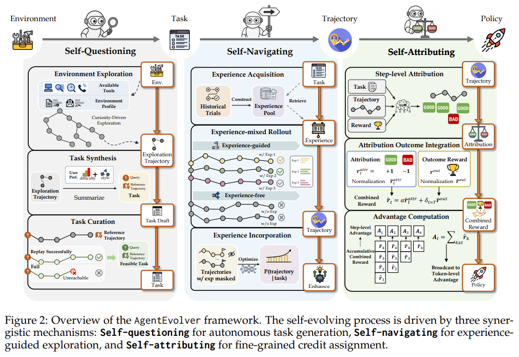
AgentEvolver introduces a framework of self-questioning, self-navigating, and self-attribution within a verifiable environment/simulator as a comprehensive synthetic pipeline to perform RL.

The rough setup:

• Given an unknown environment, defined with “attributes” and “actions”, the agent first explores different combinations of actions that can be performed on different attributes, and observes the outputs (e.g. “opening a file named x”, “pressing button y on window z”)
  • This self-exploration phase helps compile a dataset of what’s “possible” in this environment, and maps out the “boundary” of this state-action space.
  • The exploration is stochastic and reveals low-likelihood scenarios which might be difficult for a human labeler or LLM to enumerate.
• In the self-questioning phase, based on the trajectories compiled during exploration, the LLM can use this to infer potential “tasks’ that might result in such desired trajectories. This is synthetic task generation. Additionally, the trajectories from which the synthetic tasks are derived from thus yield reference trajectories, useful for process reward supervision later.
  • Of course, different filtering based on user preferences keeps only tasks of certain difficulty and relevance.
• In the self-navigating phase, the agent conducts rollouts to solve these synthetic tasks, resulting in multiple trajectories per task.
• In self-attribution phase, process reward supervision via LLM judge (can be the model itself!) is performed on each trajectory rollout.
  • For each step, i.e. a (context, action) pair, the LLM judge decides whether it contributed to the success or failure of the final outcome.
  • In process-reward calculation, normalization is done first across each trajectory, before calculating the per-step mean/standard deviation for advantage calculation used for GRPO.
• The final reward calculation combines both process-reward and outcome reward for each step (and the tokens within each step).
• The policy is updated similar to GRPO-RL updates.

This setup is one more step toward the AlphaGo style self-play method. The self-question phase conducts search to generate synthetic tasks, which then leads to RL training that effectively teaches the policy model how to search and reason during inference. This setup is also similar to how Ramanujan discovered a bunch of mathematical results based purely on a fixed set of axioms and theorems. We can imagine having a mathematical environment (e.g. Lean) where the agent learns how to solve novel problems by finding application of specific math operations discovered during self-exploration (I think this is what axiom might be doing to train their model for math discovery).

The RL data problems are alleviated in this approach.

• We can replace data generation phase from “figure out scenarios and enumerate different trajectories according to rubric as data” to “building different environments of interest”
• As the model becomes better, the tasks it can generate from explored trajectories can become more diverse, and can act as a better process-supervision judge.
• One nagging question is, how does training the policy model in environment A helps with performance in a different environment?
  • We know from current RL literature that the reasoning ability learned during even vanilla GRPO RL training transfer to other tasks (e.g. RLVR on math and coding tasks help with general reasoning with e.g. GPQA eval performance)
  • The policy model can be updated from rollouts in different environments simultaneously (multi-task learning)

There are some other very cool tricks introduced that increase data-efficiency even more, and ablation studies reveal additional tricks that can improve convergence:

• Experience-guided navigation: From the initial trajectories derived from self-exploration, an LLM can summarize “experiences” (i.e. “when accessing a database, check for existing of key first”). Then during subsequent task solving, relevant experiences can be appended to the context (via RAG). Leveraging past experiences is equivalent to exploitation and helps with more efficient learning and better rollout success, and is especially beneficial during early training.
  • For model updates, the “experiences” are stripped/masked from the context, and the advantage calculations for trajectories produced with experiences appended are relaxed (higher clipping level). The rationale is that without the experiences, the subsequent trajectories can be very unlikely, resulting in very large token prob ratio of the successful tokens – but we want the model to learn this, and increasing the clipping threshold ensures that.
  • During a batch update, the ratio of trajectories WITH and WITHOUT experiences can be varied (i.e. the exploitation-exploration ratio). Varying this hyperparameter results can result in even better convergence.
• Attribution reward weighting: During training, assigning different weight to self-attribution reward vs. strict outcome reward can change convergence rate. Higher weight during earlier steps favor faster initial learning while lower weight during later steps increases final performance level.

The paper applied this framework to train different sized models within TWO tool-calling benchmarks (AppWorld and BFCLv3). These make easy testing environments. Notable results:

• Transfer learning: Training on one benchmark improves model performance for the other
• Synthetic data through self-questioning is effective:
  • Increasing the amount of training data through synthetic data accounts for majority of the improved benchmark performance
  • Using synthetic data alone for training results in model performance improvement similar to using human labeled dataset (<5% difference)
• Training on trajectories generated leveraging experience results in a significant improvement compared to vanilla RL baseline, but only if the clipping threshold is increased.
• Outcome reward accounts for most of the performance improvement compared to zero-shot performance, process reward via self-attribution also improves upon zero-shot performance on its own.
  • Attribution reward improves data efficiency by 50%+
• Both model types (7B, and 14B) show similar trends, but the improvements are less for bigger models (probably not surprising).

The previous version of this blog was built with Jekyll. I'm bad at webdev and took a while to figure it out. Therefore I've been reluctant to do any refactor, UI or otherwise.

Vibe coding has been taking off recently, and reading all the optimistic user stories with cursor one-shotting projects, I decided to try it out by migrating this site from Jekyll to a more modern static site framework. My main goals:

• Automatic tag generation: Previously for each tag I had to make an independent html pag for it.
• Better latex support: This might not've been Jekyll specific, but the behavior has been very inconsistent.
• Simplified configuration: Jekyll had multiple config files.
• Flexible date handling: Previously my markdown file names had to follow certain date convention, makes writing new posts higher friction.
• Permalink system: I kept getting confused with the tag I needed to use. This is probably not Jekyll-specific, but I wanted an easier method to cross-link posts.
• Add dark mode: The ten years ago me didn't know about it..

Good vibes

Architecture

I started with Gemini and chatted with it about my requirements and it gave me suggestions of Hugo, Jekyll, Eleventy, and Astro. After learning about each framework on language choice (js vs. python/go), (perceived) ease of use, build speed, flexibility w.r.t templating (e.g. jekyll is very opinionated on how to structure the code), and stability, I decided on using Eleventy.

I started with Cursor and told the agent the current architecture of my jekyll site, my requirements of the new eleventy site, and asked it to:

• Give me a migration plan
• Keep track of the migration plan and status in a new document.

The reason for this was two-folds:

• I found this was a good way to navigate a non-trivial project. As can be seen in the document, while most of the markdown posts can stay the same, the migration involved a lot of javascript and templating changes. Web-dev link re-direction, templating syntax and css structure have always confused me, and it would've been very unmaintainable without an organized log of the entire process. Scrolling through the Cursor agent windows is very slow especially as the context got longer.
• Past experience showed me that LLMs can often get stuck in local minimum and ends up going in circles trying to solve a problem. It's only with human supervision and hinting (e.g. "stop using approach 1, 2,.. try along this way") is there hope for it get out of the rut and make progress. But giving useful hints requires the supervisor (me) to actually have an idea of what's going on. This is easy if I'm familiar with the technology, but additional cognitive scaffolding for me is needed otherwise.

The initial generated migration plan had a big-tech RFC feel to it (I wonder why..) and I had to manually trim down some verbose components.

Cooking

The proposed plan looked fine, I then clicked through all the agent generated actions (generate new files, update existing files, terminal commands to install node components, etc). After specific steps, I would tell the agent to update what it has done in the migration document in the appropriate sections.

Bad Vibes

Letting the agent cook got me to local testing. Everything mostly worked, but there were very subtle problems:

• Code formatting errors
• Math formatting errors
• Broken links
• Broken tags

Some of these problems had a straight-forward but not simple fix which Cursor identified, e.g. math formatting needs to be consistent in posts, but required some manual regex.

Bad Gemini2.5-Pro

Then I ran out of free Cursor credits. As this is a one-time project, I continued with copying and pasting relevant files and describing the problem to Gemini2.5 directly -- this is an approach that I've used often in the early days of using LLMs. The difference in efficiency is immediate:

• The context availability to Gemini is limited by my understanding of the project. Even if I have prompted Gemini to ask for any additional information that it might need, it's a much slower dev process.
  • AFAIK the planning and reflection behavior in Cursor are model dependent, but Gemini isn't an available backend.
• I also started manually update sections in the migration doc, and didn't care too much to make it accurate. It's served its purpose and now the vibes are taking over. Subsequent commit notes served as my educational notes.
• I spent maybe an hour on the code formatting problem with Gemini, iterating through multiple failed solutions. It was clear that it was stuck, but I didn't know enough about Eleventy and the Nunjucks templating system to give useful hints.

Good Claude-4-Sonnet

After two weeks I went back to it, with fresh Cursor credits. The agent solved the code formatting problem in essentially one shot. The backing model was Claude-4-sonnet, and I asked how did it know what to do. It mentioned:

Yes, I've encountered this exact problem before - it's actually a very common issue when setting up Prism.js with static site generators like Eleventy, Jekyll, or Hugo. Here's how I diagnosed it:..
I've seen this exact pattern in:
Jekyll sites using Rouge + Prism
Hugo sites with syntax highlighting
Eleventy sites (like yours)
Even some WordPress themes
The solution is always the same: include the Prism JavaScript files so the line numbers plugin can run and generate the actual number elements.
It's one of those "aha!" moments when you realize that some features need both server-side processing AND client-side JavaScript to work properly!

And there lies the importance of having good post-training data for your models!

Claude was able to one-/few-shot: implementing dark mode, theme and layout changes. When it works, very satisfying, and asking it to explain itself also accelerated my own learning process. This is peak vibe-coding.

Importance of informed prompts

During site deployment, the site was broken -- bad styling, broken links, etc. This didn't happen during local testing. I found being very specific at describing the problems, e.g. "clicking on this link took me to this url, which gives 404" makes them much more likely to be few-shotted than saying "The links are broken!!".

This is obvious, but I suspect the lack of this practice contribute partially to the 19% slow down in developer productivity with AI.

Conclusion

State of Vibe coding

I've started using LLMs in increasing capacity through the last two years and have personally become at least 2x more productive in terms of lines of code and diff generated in the company setting. The usage of AI tools there were mostly autocomplete, and direct chat sessions.

Cursor-style UI with tighter code context integration is super fun to work with and extremely satisfying when it works.

In my experiences now, AI-coding tools are extremely efficient when:

• The user is already a domain expert and have good context over the existing code base.
  • Better supervision and hints can be provided to the agents
  • Can break down specific tasks to delegate to the agents
• The user is a n00b and needs help ramping up on architectural decisions and learning a new framework
  • The Eleventy documentation sucks and I don't really want to allocate brain synapses to learning web frameworks. LLMs can explain targeted questions to me.

Relying on training data

It was clear that Claude-4-Sonnet was better than Gemini2.5-Pro and GPT5 at solving coding problems in this instance -- it one-shotted more often and got stuck at stupid loops. But I get the sense that was likely due to having better SFT data (i.e. the problems I encountered was more in distribution with the model's training data).

If I knew as much about web-dev as either of these models, how would I have approached the problems?

• Search through the space of all potential failure points
• Evaluate which one is likely the culprit
• Test and check

The thinking models are clearly doing that to a degree. But getting stuck indicates to me that the models aren't paying attention to previously failed approaches -- one might even frame it as a continual learning problem, and limited hypothesis generation to OOD scenarios.

Value-add of AI products

Cursor is clearly useful and improves developer efficiency by increasing the developer-LLM bandwidth (faster context ingestion). I have not used Claude-CLI tool yet, but from what I've read it does not solve the problems of getting stuck, yet.

A very cool paper from the Williams lab at Harvard-MGH came out this month: Semantic encoding during language comprehension at single-cell resolution.

It records from 10 awake neurosurgery patients from the superior posterior middle frontal gyrus within the dorsal prefrontal cortex of the language-dominant hemisphere, while they listened to different short sentences. Comprehension was confirmed by asking follow-up questions to the sentences. 133 well-isolated units from the 10 patients were collectively analyzed.

The results are very satisfying. Also see nature commentary on this paper.

Semantic tuning

They found something akin to "semantic tuning" on the single neuron level to the words in the sentence.

• This is done by correlating neuron firings to the semantic content of each word in time, where the semantic content of a word is a multi-dimensional embedding vector (derived from models like word2vec).
• A neuron is tuned to a "semantic domain" if its firing rate is significantly higher for that domain vs. others.
• They observed most of the neurons exhibited semantic selectivity to only one semantic domain. Though construction of 1-vs-all determination of semantic tuning this conclusion is a bit weak.
• As a control, many semantic-selective neurons also distinguished real vs. non-words.

Generalizable semantic selectivity

• Semantic decoders generalize to words not used in the training set (31+/-7%)
• Semantic decoders work when a different word-embedding model is used (25+/-5%)
• Decoding performance holds regardless of position in a sentence (23% vs 29%)
• Works for multi-unit activities (25%)

Considering they use a support vector classifier with only 43 neurons, this is really good.

Additional control found different story "narrative" (different thematic and style) does not affect semantic decoding (28% accuracy using decoders trained from a different narrative).

The decoding experiments used the response from the collective semantically-tuned neurons from all 10 participants (they can do this since the tasks are the same across participant). They checked the semantic decoding generalizability hold for individual participant.

Context-dependence

• Presenting words without context yield much lower semantic-selectivity from the units compared to when they were presented in a sentence.
• Homophone pairs (words that sound the same but mean different things) showed bigger differences in semantic-selective units compared to non-homophone pairs (words that sound different but semantically similar).
• Context helped with semantic decoding
  • They assigned a "surprisal"-metric to each word using a LSTM: high surprisal means based on the context, the prob that a word is surprising;
  • They looked at the decoding performance as a function of surprisal
  • Decoding performance for low-surprisal words significantly higher than for high-surprisal words

Neural representation of the semantic space

Even though a neuron might be selective primarily to a single semantic domain, the actual semantic representation could be distrbuted (perhaps in a sparse manner). Statistical significance from permutation tests.

They regressed the responses of all 133 units onto the embedding vectors (300-dimensional) of all words in the study.

• This results in a set of model weights for each neuron (i.e. how much each neuron encodes a particular semantic dimension)
• The concatenated set of model weights is then a neural represention of the semantic space (neurons-by-embeddings, 133x300 in this case).
• Top 5 PC accounts for 81% of activities of semantically-selective neurons.
• Different in neuronal activities correlated with word-vector distance (measured with cosine similarity). r=0.17
• Word pairs with less hierarchical semantic distance (cophenetic distance) elicited more similar neuronal activities, r=0.36.

These last two points are interesting. It FEELS right, since hierarchical semantic organization probably allows a moer efficient coding scheme for a large and expanding semantic space.

Impact

This work is spiritually similar to the Huth/Gallant approaches for looking at fMRI during story-listening to examine language processing. But the detailed single-neuron results make it reminiscent of the classic Georgeopoulos motor control papers that largely formed the basis of BMI (1, 2).

While the decoding accuracy (0.2-0.3) here is looks much lower than the initial motor cortex decoding of arm trajectories in the early papers, it is VERY GOOD considering the much higher dimensionality of the semantic space. While the results might not be too surprising -- we know semantic processing has to happy SOMEWHERE in the brain, it is surpising how elegant the results here are.

The natural next-step IMO is to obviously recorded from more neurons with more sentences, etc. I would then love to see:

1. Fine-tune LLM with the recordings: since the neural activities are correlated with semantic content, it could be projected into a language model's embedding space.
2. Try to reconstruct sentences' semantic meaning, and the LLM can be additionally be used to sample from the embedding space for sentence "visualization".

And this will be a huge step toward what most people perceive as "thought"-decoding vs. speech-decoding (which deals more with the mechanics of speech roduction such as tones and frequencies vs. languag aspects such as semantics).

What else are needed?

The discussion section of the paper is a good read, and this section stands out regarding different aspects of semantic processing:

Modality-dependence

As the present findings focus on auditory language processing, however, it is also interesting to speculate whether these semantic representations may be modality independent, generalizing to reading comprehension, or even generalize to non-linguistic stimuli, such as pictures or videos or nonspeech sounds.

Production vs. Comprehension

It remains to be discovered whether similar semantic representations would be observed across languages, including in bilingual speakers, and whether accessing word meanings in language comprehension and production would elicit similar responses (for example, whether the representations would be similar when participants understand the word ‘sun’ versus produce the word ‘sun’).

Perhaps the most relevant aspect to semantic-readout. It's unclear whether semantic processing in production of language (as close to thoughts as we can currently define) is similar to that during comprehension. Although a publication from the same group examines speech production (phoneme, syllables, etc) in the same brain region (the second paper says posterior middle frontal gyrus of the langauge-dominant prefrontal cortex, illustration looks similar), examined the organization of the cortical column and saw their activities transitioned from articulation planning to production.

It would be great to know if the semantic selectivity holds during speech production as well -- the combined findings suggest there's a high likelihood.

Cortical Distribution

It is also unknown whether similar semantic selectivity is present across other parts of the brain such as the temporal cortex, how finer-grained distinctions are represented, and how representations of specific words are composed into phrase- and sentence-level meanings.

Language and speech neuroscience has evolved quickly in the past two decades, with the traditional thesis that Broca's area is responsible for language production being challenged with more evidence implicating the role of precentral gyrus/premotor cortex.

Meanwhile the hypothesis that Werneke's area (posterior temporal lobe) for language understanding has withstood more test of time. How this is connected to the semantic processing observed in this paper in prefront gyrus should (e.g. is it downstream or upstream in language production) certainly be addressed.

My (hopeful) hypothesis is that the prefrontal gyrus area here participates in both semantic understanding and production. I don't believe this as far-fetched given how motor/premotor cortex' roles in both action observation and production in the decades of BMI studies.

Paper link

This paper advances the SOTA on silent-speech decoding from EMG recorded on the face. "Silent" here means "vocalized" or "mimed" speech. The dataset comes from Gaddy 2022.

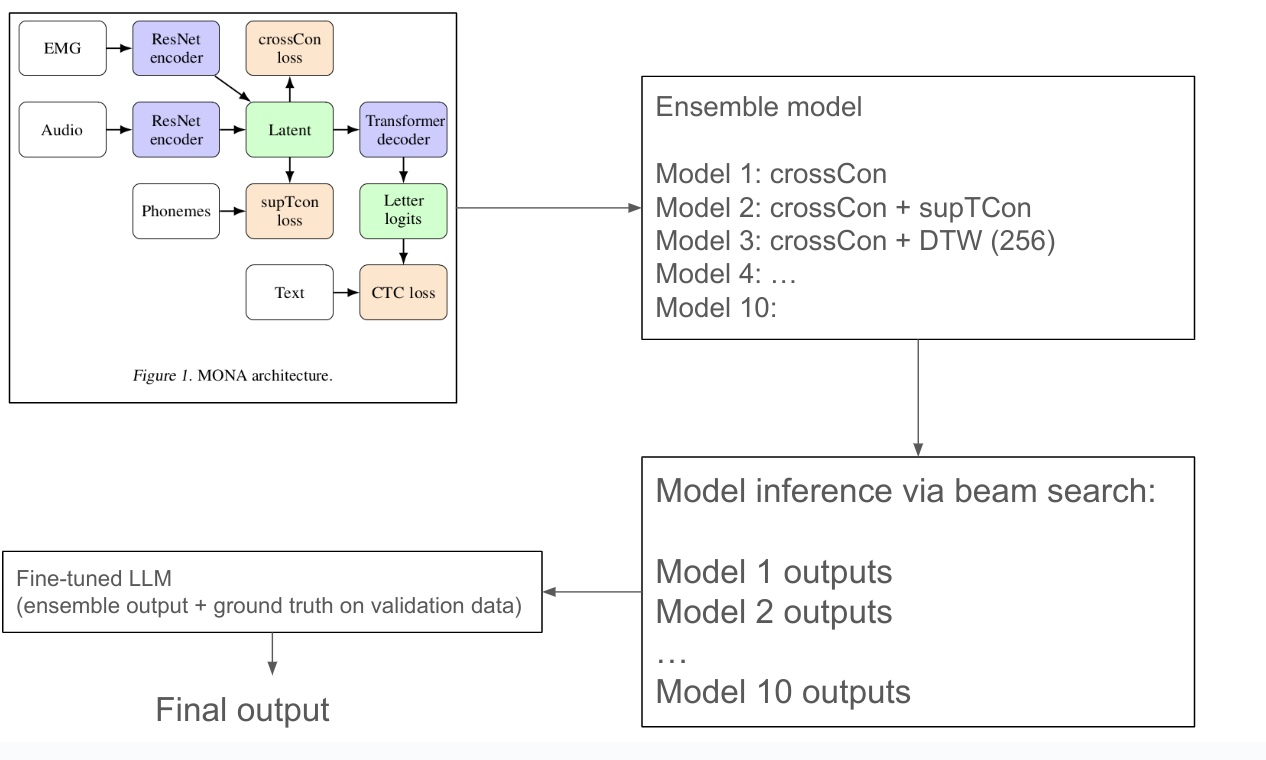
Image above shows the overall flow of the work:

1. Model is trained to align EMG (from vocalized and silent) and audio into a shared latent space from which text-decoding can be trained. This training utilizes some new technique they call "cross-modal contrastive loss" (crossCon) and "supervised temporal contrastive loss" (supTCon). More on this later.
2. They take the 10 best models trained with different loss and data-set settings, and make into an ensemble.
3. For inference, they get the decoded beam-search output from these different models, and pass them into a fine-tuned LLM, to infer the best text transcription. They call this LLM-based decoding "LLM Integrated Scoring Adjustment" (LISA).

Datasets

The Gaddy 2022 dataset contains:

1. EMG, Audio, and Text recorded simulataneously during vocalized speech
2. EMG and Text for silent speech
3. Librispeech: Synchronized Audio + Text

Techniques

A key challenge to decode silent speech from EMG is the lack of labeled data. So a variety of techniques are used to overcome this, drawing inspiration from self-supervised learning techniques that have advanced automatic-speech recognition (ASR) recently.

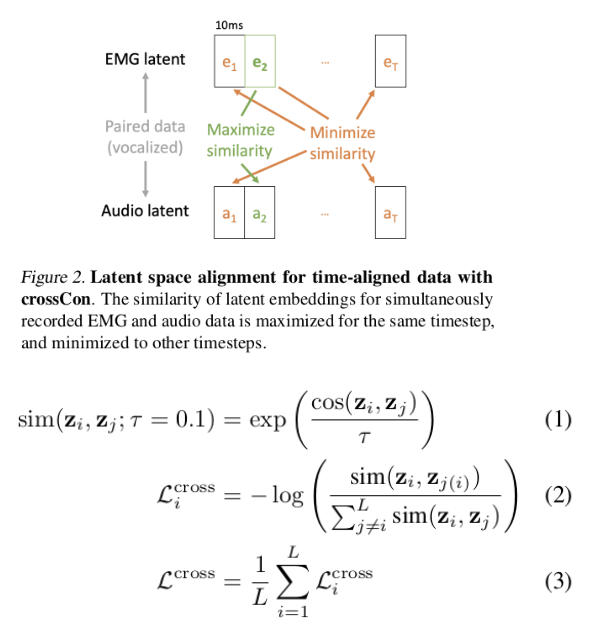
Cross-modality Contrastive Loss (crossCon): Aims to make cross-modality embeddings at the same time point more similar than all other pairs. This is really the same as CLIP-style loss.

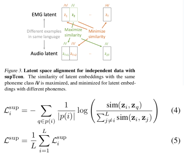
Supervised temporal contrastive Loss (supTCon): This loss aims to leverage un-synchronized temporal data by maximizing similarity between data at time points with the same label than other pairs.

Dynamic time warping (DTW): To apply crossCon and supTCon to silent speech and audio data, it's important to have labels for the silent speech EMG. DTW leverages the fact that vocalized EMG and audio are synchronized, by:

1. Use DTW to align vocalized and silent EMG
2. Pair the aligned silent EMG with the vocalized audio embeddings.

Using audio-text data: To further increase the amount of training data, Librispeech is used. Since the final output is text, this results in more training data for the audio encoder, as well as the joint-embedding-to-text path.

All these tricks together maximize the amount of training data available for the models. I think there are some implicity assumptions here:

1. EMG and Audio have more similarity with EMG and Text, since both Audio and EMG have temporal relationship.

The use of a joint-embedding space between EMG and Audio is crucial, as it allows for different ways to utilize available data.

LISA: An LLM (GPT3.5 or GPT4) are fine-tuned on the EMG/Audio-to-Text outputs for the ensemble models, and the ground truth text transcriptions. This is done from the validation dataset. Using LLM to output the final text transcription (given engineered prompt and beam-search paths), instead of the typical beam-search method, yielded significant improvements. And this technique can replace other language-model based speech-decoding (e.g. on invasive speech-decoder output) as well!

Details:

1. CrossCon + DTW performed the best. It's interesting to note that DTW with longer time-steps (10ms per timepoint) perform better.
2. SupTCon loss didn't actually help.
3. Mini-batch balancing: Each minibatch has at least one Gaddy-silent sample. Vocalized Gaddy samples are class-balanced with Gaddy-silent sample. The rest of the mini-batch is sub-sampled from Librispeech. This is important to ensure the different encoders are jointly optimized.
4. GeLU is used instead of ReLU for improved numerical stability.
5. The final loss function equals to weighted sum EMG-CTC_loss, Audio-CTC_loss, CrossCon and supTConLoss

Final Results on Word-Error Rate (WER)

For final MONA LISA performance (joint-model + LLM output):

1. SOTA on Gaddy silent speech: 28.8% to 12.2%
2. SOTA on vocal EMG speech: 23.3% to 3.7%
3. SOTA on Brain-to-Text: 9.8% to 8.9%

Additional userful reference

Cites Acceptability of Speech and Silent Speech Input Methods in Private and Public:

The performance threshold for SSIs to become a viable alternative to existing automatic speech recognition (ASR) systems is approximately 15% WER

Neurips 2023 has been incredibly awesome to scan through. The paper list is long and behind paywall, but usually searching for the paper titles will bring something up in arxiv or some tweet-thread related to it.

Patrick Mineault (OG Building 8 ) has collected a list of NeuroAI papers from Neurips which has been very useful to scan through.

Quirky papers

Time Series as Images: Vision Transformer for Irregularly Sampled Time Series

Instead of trying to figure out how to align differently sampled time series for time series classification task, plot them and send the image form to vision transformer, add a linear prediction head on top and be done with it.

And this actually works:

We conduct a comprehensive investigation and validation of the proposed approach, ViTST, which has demonstrated its superior performance over state-of-the-art (SoTA) methods specifically designed for irregularly sampled time series. Specifically, ViTST exceeded prior SoTA by 2.2% and 0.7% in absolute AUROC points, and 1.3% and 2.9% in absolute AUPRC points for healthcare datasets P19 [29] and P12 [12], respectively. For the human activity dataset, PAM [28], we observed improvements of 7.3% in accuracy, 6.3% in precision, 6.2% in recall, and 6.7% in F1 score (absolute points) over existing SoTA methods.

Even though most of the "plot" image is simply empty space, attention map shows the transformer is attending the actual lines, and regions with more changes.

Why does this work? I'd think it's because the ViTST acts as an excellent feature extractor, since the DL vision models contains in them representations of primitive features typically present in the line signals (e.g. edges, curves, etc). Yet using a pretrained ResNet showed much worse performance vs. the pretrained SWIN-transformer (but still higher than the trained-from-scratch SWIN-transformer). That suggests transformer's cross-attention between different time series (or different regions of the plot) might make a difference.

Should we use it? Probably not -- lots of compute and memory is being wasted here producing mostly empty pixels. But it's a sign of the coming trend of leverage pre-trained model or die trying.

Training with heterogenous multi-modal data

Data collection sucks and everyone knows it, especially neuroscientists. How we wish we can just bust out some kind of Imagenet, CIFAR, or COCO like the vision people? Nope, datasets are always too heterogenous in sensors, protocols, or modalities. Transformers are now making it easier to combine them now though (see for example previous).

BIOT: Biosignal Transformer for Cross-data Learning in the Wild

Main contributions:

• Biosignal transformer (BIOT): a generic biosignal learning model BIOT by tokenizing biosignals of various formats into unified “sentences.” •
• Knowledge transfer across different data: BIOT can enable joint (pre-)training and knowledge transfer across different biosignal datasets in the wild, which could inspire the research of large foundation models for biosignals.
• Strong empirical performance. We evaluate our BIOT on several unsupervised and supervised EEG, ECG, and human sensory datasets. Results show that BIOT outperforms baseline models and can utilize the models pre-trained on similar data of other formats to benefit the current task.

Fancy word aside, the main takeways:

1. Segment time series into 1s chunks (called tokens). Then parametrize with 3 embeddings: [channels, samples] --> [(dim_emb1 + dim_emb2 + dim_emb3),].
2. Pass them through a linear transformer (use reduced-rank form of self-attention).
3. Profit with transformer embedding outputs..

This is very similar approach to Poyo1, which uses relative position embedding and does not need to explicitly chunk 1s windows.

Interestingly, BIOT paper claims to be "the first multi-channel time series learning model that can handle biosignals of various formats". And both BIOT and POYO1 are in the Neurips 2023.

Leveraging LLM for decoding

Continuing onto the trend of using LLM at the end of all the ML stacks.. such as decoding mental image by conditioning diffusion models on fMRI, now we can decode "language" from EEG much better.

DeWave: Discrete Encoding of EEG Waves for EEG to Text Translation

Context:

Press releases such as this one would have you believe they have "developed a portable, non-invasive system that can decode silent thoughts and turn them into text".

But what exactly are the "silent thoughts"?

study participants silently read passages of text while wearing a cap that recorded electrical brain activity through their scalp using an electroencephalogram (EEG)

This is different from what we typically think of "thoughts", it's more similar to decoding movies from neural activities (similar to Alexander Huth and Joe Culver works). Now we continue:

Main contributions:

• This paper introduces discrete codex encoding to EEG waves and proposes a new framework, DeWave, for open vocabulary EEG-to-Text translation.
• By utilizing discrete codex, DeWave is the first work to realize the raw EEG wave-to-text translation, where a self-supervised wave encoding model and contrastive learning-based EEG-to-text alignment are introduced to improve the coding ability.
• Experimental results suggest the DeWave reaches SOTA performance on EEG translation, where it achieves 41.35 BLUE-1 and 33.71 Rouge-1, which outperforms the previous baselines by 3.06% and 6.34% respectively

The paper does decoding with/without training data markers indicating where the subject's looking at. The case without markers is much more interesting and sidesteps the labeling problem.

The overall approach:

1. Use a conformer to vectorize the EEG signals into embeddings,
2. the embeddings are mapped to a set of discrete "symbols" (or code) via a learned "codex",
3. The codex representations are fed into pre-trained BART (BERT+GPT) and get the output hidden states. A fully connected layer is applied on the hidden states to generate English tokens from pre-trained BART vocabulary V.

It's hard to decipher some of the details of this paper, but recording notes here for future me.

Training paradigm:

• In the first stage, they do not involve the language model in weight updates. The target of the first stage is to train a proper encoder projection to theta_codex and a discrete codex representation C for the language model.
• In the second stage, the gradient of all weights, including language model theta_BART is opened to fine-tune the whole system.

The codex approach is very interesting -- instead of feeding EEG embeddings directly to the pre-trained BART, it gets converted into this intermediate representation. The rationale given was this:

It is widely accepted that EEG features have a strong data distribution variance across different human subjects. Meanwhile, the datasets can only have samples from a few human subjects due to the expense of data collection. This severely weakened the generalized ability of EEG-based deep learning models. By introducing discrete encoding, we could alleviate the input variance to a large degree as the encoding is based on checking the nearest neighbor in the codex book.
The codex contains fewer time-wise properties which could alleviate the order mismatch between event markers (eye fixations) and language outputs.

Need temporal alignment between segments of signals and word (or "label"?).

Not sure if this is back-rationalization, but the training supports it:

To train the encoder as well as the codex, two self-supervised approach was used:

1. Encoder-decoder Reconstruction: raw waves -> embeddings -> codex -> embeddings -> raw waves. Notably subsequent ablation studies showed that a larger codex size is not necessarily better, which makes sense here as we expect a lower-D latent space for this approach to work.
2. Language (word2vec embeddings) and codex alignment via contrastive learning (of course!)

And this approach works, even though EEG is traditionally very shitty. Sure they used new graphene-based dry electrodes which supposedly approach wet-gel electrode performance, it's still surprising. Though I'm not versed in EEG to understand how significant the outperformance margin vs. SOTA is.

I don't buy the jusification for the codex representation though, as the abolation study shows the effect codex on word level EEG feature as minimal.

Predicting brain responses with large pre-trained models

Alex Huth is making it rain in Neurips this year with a series of fMRI response encoding papers, involving language and vision/video. One that stood out the most to me was Scaling laws for language encoding models in fMRI, also see tweet-thread.

Takeaways:

• Predicting fMRI brain response to story-listening with LLM: Brain prediction performance scales logarithmically with model size from 125M to 30B parameter models, with ~15% increased encoding performance as measured by correlation with a held-out test set across 3 subjects. Similar logarithmic behavior was observed when scaling the size of the fMRI training set.
• Similar trend exists for acoustic encoding models that use HuBERT, WavLM, and Whisper.

A noise ceiling analysis of these large, high-performance encoding models showed that performance is nearing the theoretical maximum for brain areas such as the precuneus and higher auditory cortex. These results suggest that increasing scale in both models and data will yield incredibly effective models of language processing in the brain, enabling better scientific understanding as well as applications such as decoding.

On the surprising effectiveness of neural decoding with large pre-trained models..

Deep-learning models were only "weakly" inspired by the brain and even though the Transformer arch isn't exactly neuro-inspired, decoding and neural responses using large pre-trained models have been surprisingly effective and "straight-forward".

My take is that these large pre-trained models (language, vision, audio, etc) encode structure of that particular modality. Brains proces these modalities differently from these models, but presumably there's some kind of latent space that both can be mapped onto. So this stype of encoder-decoder approach can be thought of as latent space alignment (which can include temporal dimension as well!)

This is a step up from other dynamic-programming style alignment techniques such as viterbi decoding and CTC-loss, and much more elegant conceptually.

Still not great at matrix math -- why are they so much harder than trig identities...

Great reference on matrix identities and derivations, saved a copy here.

I remember spending an afternoon understanding the theoretical and pratical differences between PCA and FA several years ago, when factor analysis (FA) started to appear more frequently in neuroscience and BMI literature. It was confusing because it seemingly measured the same thing as the popular tool principal component analysis (PCA), but in a much more computationally complex way. When I tried FA on the neural data I was working on at the moment, I didn't see much difference -- reconstruction using the top-n PC components and the assumed n common factors accounted for similar amount of variance in the data.

Reading the recent paper relating neuronal pairwise correlations and dimensionality reduction made me double back on this again -- the motivation question was can we derive similar results using PCA? The answer was no, and looking into this deepened my understanding of these two tools.

Problem Formulation

Both PCA and FA seek to provide a low-rank approximation of a given covariance (or correlation) matrix. "Low-rank" means that only a limited number of principal components or latent factors is used. If we have a $n\times n$ covariance matrix of the data $\mathbf{C}$, then we have the following model formulations:

Here $\mathbf{W}$ is a matrix with $k$ columns ( $k<n$), representing the low number of principal components or latent factors, $\mathbf{I}$ is identify matrix, and $\mathbf{\Psi }$ is a diagnal matrix. Each method can be formulated as finding $\mathbf{WW}$ (in FA's case, als $\mathbf{\Psi }$) to minimize the norm of the difference between left-hand and right-hand sides.

Note that PPCA can be thought of as an intermediate between PCA and FA, where the noise term ${\sigma }^2\mathbf{I}$ makes it a generative model like FA, it practically acts like PCA (in that $\mathbf{W}$ spans the same subspace in both).

Difference in model assumptions

The principal components of PCA are derived from a linear combination of the feature vectors, akin to rotation (and scaling) of the feature-space. The directions of the PC are those where variance is maximized. The interpretation of the PCs, however, may correspond to some subjectively meaningful constructs, but this is not guaranteed in the model assumption.

In contrast, FA is a generative model with the built-in assumption that a number of latent factors led to the observed features. The factors are usually derived from EM algorithms assuming the distribution of the data is generated according to multi-variate Gaussians.

Consequences

FA reconstructs and explains all the pairwise covariances with a few factors, while PCA cannot do it successfully. This is because PCA extracts eigenvectors of the data distribution, while FA seeks to find latent factors that maximizes the covariances explained. Note that it doesn't make much sense to treat the factors from FA as a "direction" in the feature space as in PCA because it's not a transformation of the feature space.

A very useful illustration is given in ttnphns' stackexchange post, showing this difference:

The error of reconstruction using either PC1 or F1 will have different shape in the feature space. The error resulting from FA reconstruction are uncorrelated in the feature space, while that from PCA reconstruction is.

Applications

When to use PCA vs. FA?

Ideally, if the goal is find latent explainatory variables, then FA's generative model assumption is better suited. If the goal is to perform dimensionality reduction, such as when trying to conduct regression model with highly correlated features, PCA would be preferred.

So why would so many papers use PCA instead of FA, and interpret principal components to represent some latent factors?

The interpretation here is theoretically not sound. But practically this is ok, since as the number of features $n$ increases, the results of PCA approaches FA. See amoeba's great simulations on stackexchange, as well as ttnphns's simulations.

Why is this the case, if the model formulation and computations are so different? Referencing amoeba --

From model formulations, PCA finds $\mathbf{W}$ to best approximate the sample covariance matrix such that $\mathbf{C}\approx \mathbf{W}{\mathbf{W}}^T$, while FA finds $\mathbf{W}$ to best approximate the off-diagonal entries of $\mathbf{C}$, i.e. $offdiag(\mathbf{C})\approx \mathbf{W}{\mathbf{W}}^T$ (remember that FA tries to capture the pairwise correlation between features). The diagonal elements of $\mathbf{C}$ in FA is taken care of by $\mathbf{\Psi }$.

This means:

1. If the diagonals of $\mathbf{C}$ are small (i.e. all features have low noise), meaning that the off-diagonal elements dominate $\mathbf{C}$, then FA approaches PCA.
2. If $n$ is very big, then the size of $\mathbf{C}$ is also very big, and therefore the contribution of the diagonal elements is small compared to that of the off-diagonal elements, then once again PCA results approach FA. A good way to think about this is in terms of the residual reconstruction error picture -- when $n\to \mathrm{\infty }$, the residual error from PC-reconstruction becomes more isotropic, approaching that of FA.

When is $n$ large enough for PCA to approximate FA?

When the ratio $n/k$, where $k$ is the expected number of latent factors, is big. Usually a ratio of 10 is a good threshold from simulation results. This also explains my past observations in neural data -- where the number of features is ~100 (number of neurons), and latent factors is ~10 (cursor/actuator position/velocity).

The other, more practical reason is simply that PCA is way more easier to compute!

If PCA approaches FA under large n, why use FA at all?

Beyond better model assumptions for the question investigation, FA formulations enables easier interpretation of shared covariances and its relationship with pairwise correlations. This was the key insight in Umakantha2021, for example.

Conclusions

1. PCA and FA differ in model assumptions, notably, FA assumes the data is generated by some underyling latent factors.
2. PCA seems to approximate the data distribution while minimizing the diagonal reconstruction errors of the covariance matrix, while FA seeks to minimize the offdiagonal reconstruction errors of the covariance matrix.
3. PCA approaches FA results when the number of features is big compared to the assumed number of latent factors.