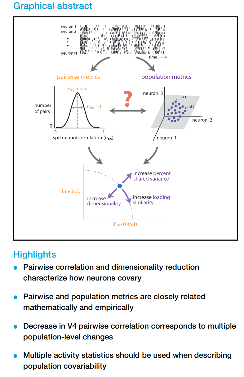
Pairwise correlations between individual neurons, and dimensionality reduction based methods to characterize population statistics are widely used to measure how neural populations covary. This paper establishes mathematical relationships between the two approaches and demonstrate that summarizing population-wide covariability using any single activity statistic is insufficient.
The graphical abstract and highlights on the publication are actually very informative after reading through some of the paper:
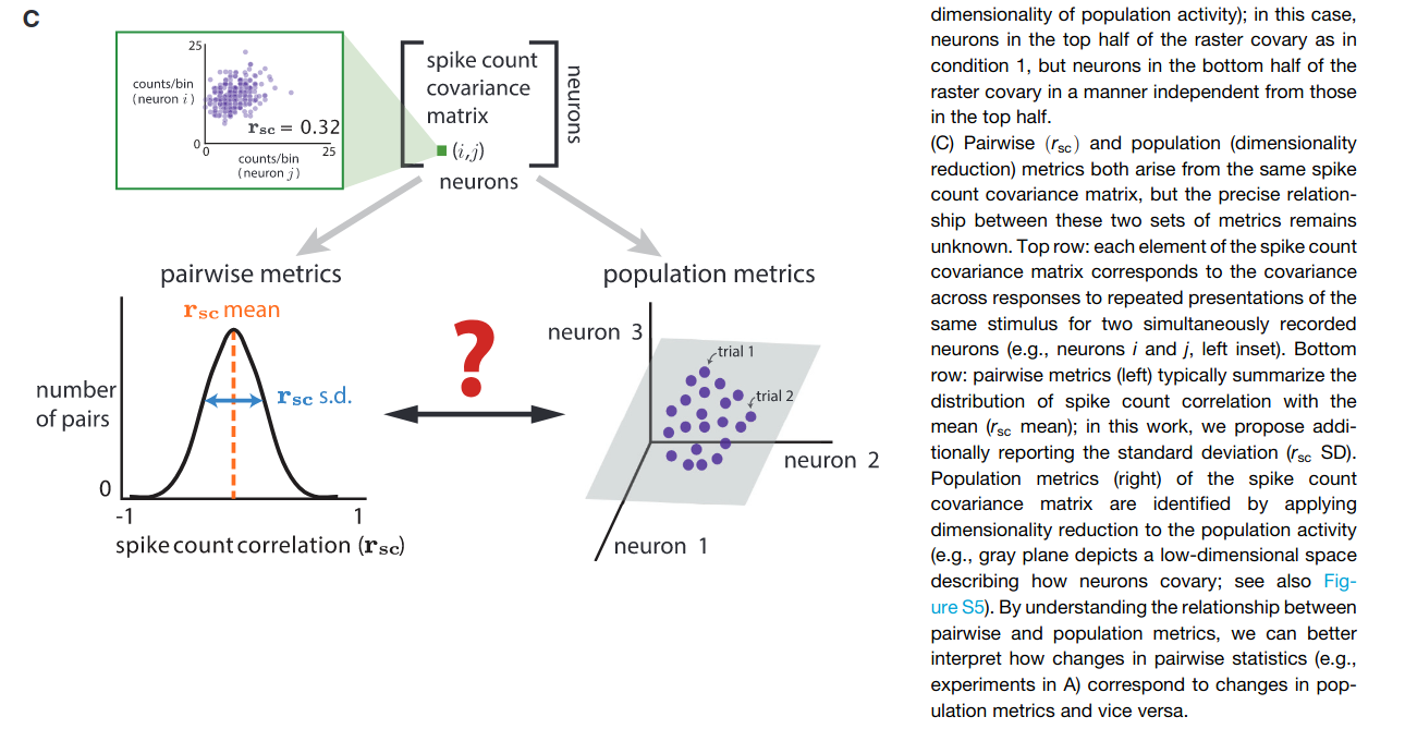
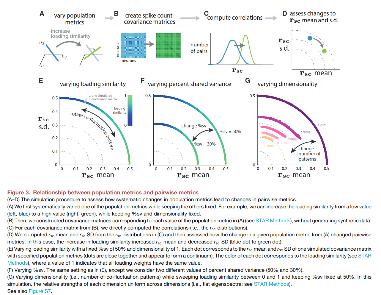
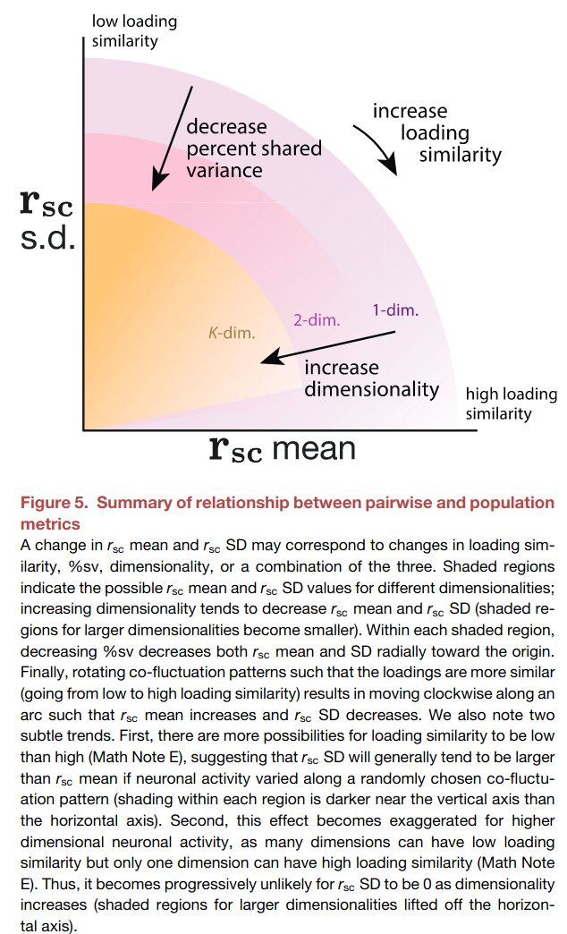
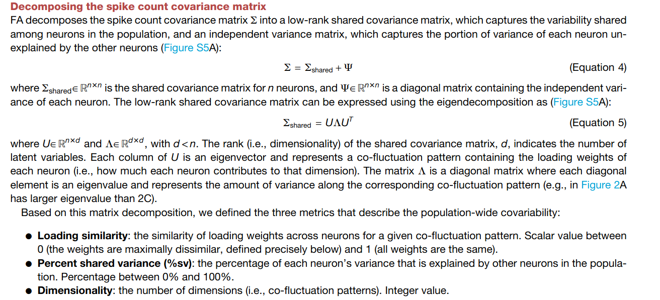
As is typical Byron Yu/Aaron Batista fashion, this paper presents a clever application of dimensonality reduction (specifically factor analysis).
Neuroscience literature often presents pairwise statistics to characterize neural populations (i.e. average spike-count correlations before and after learning BMI). They first propose that that this measure needs to be complemented by the pairwise metric standard-deviation , then connect how the changes in this pair of pairwise metrics relate to population-level metrics obtained through dimensionality reduction.
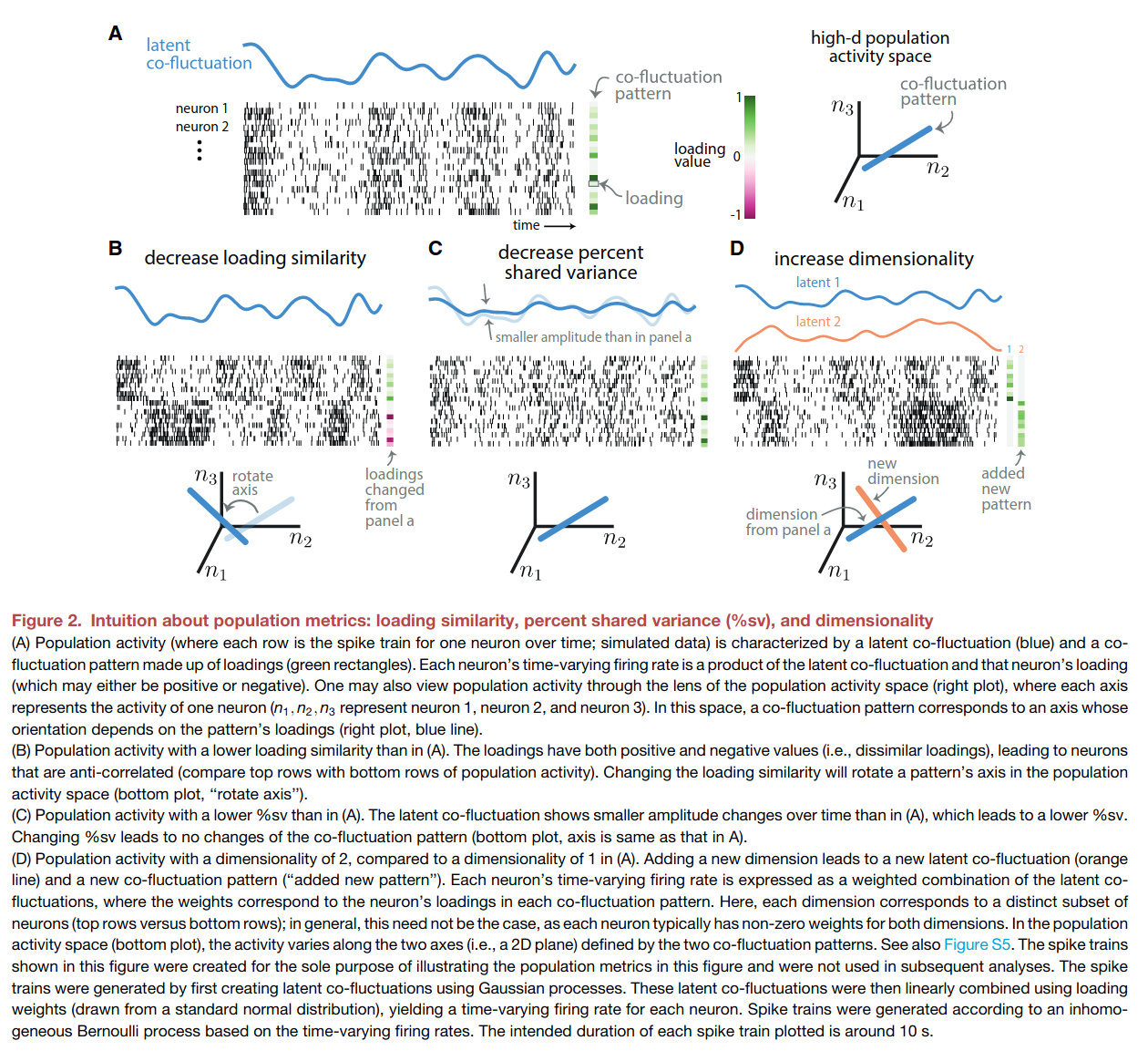
The next three figures illustrate the population-level metrics, and their relationship with pairwise metrics. The central idea is that the population activity can have different degree of covariation, which can be decomposed into shared variation along a number of latent fluctuations.
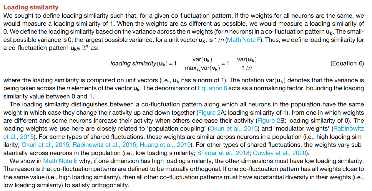
Loading similarity: How correlated population activities are.
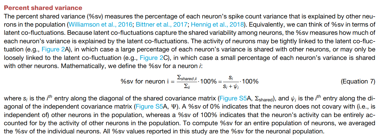
Percent-shared variance: How much each neuron's fluctuatons is captured by the latent co-fluctuation.
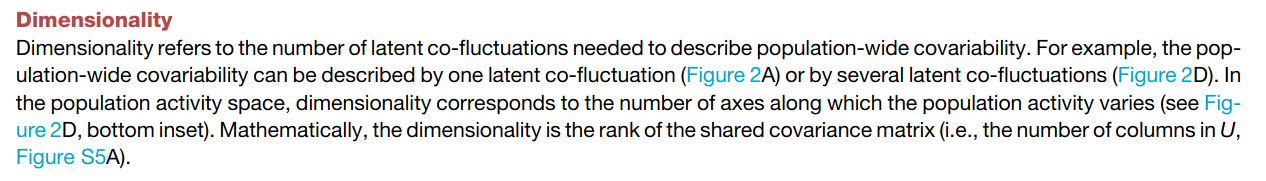
Dimensionality: The number of "co-fluctations" needed to capture the variance in the population activities (similar to number of PCs in PCA).
If all these sounds like factor analysis (FA), that's because it's a different way of interpreting F.A. The crux of the paper below:
The field of DSP is pretty broad, but I found knowing/remembering the following basic concepts are both useful in practice, and in interviews (giving or receiving). Understanding the concepts below can also make debugging unexpected results much easier, and I've had to come back to these concepts many times.
FIR vs. IIR filters
FIR filters are easy to implement, always causal.
IIR filters are more concise to implement, but it requires feedback. Can implement higher order IIR filters with biquad structures (SOS-implementations) for stability (not needed for FIR).
FIR filters are always linear phase.
IIR filters can try to be linear phase within the passband.
Phase Delay
Linear phase is when the phase-shift introduced to different frequencies are linearly increasing.
This means higher-frequency signals are delayed more in phase.
The result is that all frequencies are delayed the same in time, despite differently in phase.
Intuitively, linear phase means the filtered signal will have similar shape as before.
This phenomenon stems from the assumption of DFT, that the input signal is ONE PERIOD of a PERIODIC SIGNAL.
If the part of the signal that is windowed is not an integer multiple of the periodic signal, then the resulting frequency spectrum may not have frequency bins corresponding exactly to the frequency of interest -- the resulting DFT is not sharp, and
The frequency of interest is "spread" out into the surrounding frequency bins. producing a "leakage".
This can be solved with "zero-padding", adding zeros to the end of the time-domain signal. This approximates the effect of taking the CTFT of a windowed periodic signal.
The result is that the DFT of this zero-padded signal looks like an interpolation of the previously "spread-out" DFT of the non- zero-padded signal. For signal with a single tone, this would recover the correct peak frequency.
Zero-padding does not improve frequency resolution (interpolation doesn't increase resolution). To improve resolution we need longer duration recording of the signal.
FFT^2 vs. PSD of a signal
PSD usually applies to a stochastic process (usually stationary). For non-stationary processes such as speech, STFT should be used.
Wiener-Khinchin Theorem: For stationary stochastic process, PSD is defined as the Fourier Transform of the Autocorrelation Sequence of the signal. From this we get the amount of power per frequency bin.
PSD can be estimated by taking the magnitude squared of the FT of the signal -- this is called the Periodogram.
This is not a consistent estimator as it does not tend to a limit with increasing sample size, as the individual values are exponentially distributed.
An alternative is to get a truncated version of the auto covariance signal, then take the Fourier Transform.
This leads to spectral window of some width, has lower sampling variability and with minor assumptions IS a consistent estimator.
The key weakness of the periodogram is that it takes only one "realization" of a stochastic process and therefore has high variability..
The PSD can be thought of as a random variable -- you need to average over many outcomes to get a decent estimate
In fact, another definiton of PSD is "an average of the magnitude squared of the Fourier Transform".
Very CHEAP computationally, but has high variance.
Consequently, averaging multiple peridograms can approach the PSD.
The unit of PSD is /Hz. Integrating PSD over a delta of frequency bin gives the energy (Watts).
For a mean-zero signal, integral of the entire PSD is equal to the variance.
Key Duality: a quadratic quantity in the frequency domain (energy spectral density in determinstic case, power spectral density in the stochastic case) corresponds to a correlation (which is essentially a convolution) in the time domain.
Multi-taper approach Is a fancy way of averaging periodograms. It averages a pre-determined number of periodograms obtained by different window (taper) on the same signal. The windows selected have two key properties:
The windows are orthogonal, this means that the periodgrams are uncorrelated, so averaging multiple peridograms give an estimate with lower variance than using just a single taper.
The windows have the best possible concentration in the frequency domain for a fixed signal length to minimize spectral leakage.
Probably the best estimator for stationary time-series that's not super long..
Informative resource with a good discussion on why so many PSD calculations: 1
Savitzky-Golay filter
I actually haven't encountered this in grad school, probably because I dealt mostly with spikes, and didn't need the smoothing abilities that SGF is especially suited for. Everyone in my job seems to love it for some handwavy reason so I wanted to demystify it. A good overall discussion of the pros/cons beyond the basic formulation is on stackoverflow. Some highlights:
Let's get it straight, SGF is not magical, adaptive or anything. It's an FIR filter designed with local polynomial approximation.
If the noise spectrum significantly overlaps with the signal spectrum, a more careful approach is required, and brute-force attenuation will not work well because either you leave too much noise (by choosing the cut-off frequency too high) or you distort the desired signal too much. In this case Savitzky-Golay (S-G) filters may be a good choice.
Can be thought of a FIR low-pass filter, with flat passband, and moderate attenutation in the stop band.
Good for preserving peak shapes and height, bad for rejecting noise.
Use when you want to smooth, but the noise and signal share similar frequency.
SGF with smaller window length means less attenuation in higher frequencies, this means it distorts the peaks less, but noise that's slightly out of the band are not filtered as sharply.
Longer window attenuates more, but keeps the amplitude constant for a basic sinusoid.
Examples/Tests:
Clean signal of 1Hz, corrupt with 10Hz, and 40Hz (yes the noise are out of band). Len-31 sgf would perform better than len-101 because it distorts the peaks less, and the resulting waveform is almost identical to the base 1Hz waveform.
Clean signal of 1Hz, corrupt with 1.2Hz and 40Hz. Len-31 sgf results in a smoother version of the original signal. Len-101 sgf results in a 1Hz signal with smaller amplitude. In this case, Len-101 correctly filtered out the high frequency components better.
In practice, I actually found SGF to be hard to use/tune. Much better to do actual adaptive filtering (e.g. H-infinity, LMS) if a noise measurement is available.
Utilizing ergodicity to increas SNR
In diffusion correlation spectroscopy, for example, SNR is proportionally to photon rate (more signal per time), and integration time (for more accurate auto-correlation calculation).
However, more than one measurement can be taken at a time, increasing the number of measurements spatially can then achieve similar SNR increase as a greater photon rates and/or integration time.
This is based on the assumption of ergodicity -- i.e. a random process averaged over time/space has the same mean and variance.
Time Series ARIMA models and Signal Processing relations
Every autoregressive-integrated-moving-average (ARIMA) model can be converted to an infinte order MA model -- similar to how IIR filters can be approximated by FIR filters!
When decomposing (trend + seasonal + random) additive models, trend is extracted by sliding window centered moving averages (similar to low-pass filtering), with a window length equal to the seasonal span.
Smoothing: LOWESS/LOESS are equivalent to Savitzky-Golay -- i.e. fitting regressions or polynomials locally to each point, may include weighting function applied to different points.
We shouldn't blindly apply exponential smoothing because the underlying proces smight not be well modeled by an ARIMA(0,1,1). The reason is that Exponential Moving Average (EMA) is equivalent to a first-order moving average (MA1) model.
Diagnostics:
AR models should show decaying autocorrelation function (ACF) and cutoff in partial autocorrelation function (PACF).
MA models should show cutoff ACF, and decaying PACF.
ACF and PACF both showing spike-cutoff patterns suggests ARIMA model.
Seasonal trends show periodic cutoff ACF or PACF
How to fit ARIMA model to linear model residuals:
Cochrane-Orcutt (example) does pre-whitening, then apply OLS to get the beta coefficients and SE. R-squared after this procedure is ususually less than that of LS
ARIMAX: Fitting regression with ARIMA error structure, can be done with Cochrane-Orcutt, but better with maximum-likelihood estimation to joint estimate both the regression model and error ARIMA model.
Can treat this as a state-space model -- the ARIMA error describes the state transition, the exogeneous regressors describe the observation model.
Some connection to Kalman filtering after some manipulations.
Yule-Walker...because I can never remember this name..
Order structure is determined by maximum-likelihood or AIC of the fit to the residuals.
Wiener-Hopf equation is a generalization of the Yule-Walker equations.
DSP-implementation gotchas:
SOS/biquad implementation are better than transfer function implementations in practice due to robustness in overflow and quantization error. For example, see scipy issue.
When implementing cascade of filters in DSP, it's important to think about and set the initial conditions for the 2nd stages and on. These filter stages should have initial condition set to the step response steady-state of the previous filter, corresponding to that state's initial state, and so on.
My newest hobby is high-altitude mountaineering. There's so much different advices out there about how to improve endurance and speed, to go faster for longer. Information from runners and climbers and cyclists can be very different.
I got nerdy and dug into the physiology and evaluated the main training methods:
To find which one or combination is the most optimal training solution for climbing big mountains, along with other training techniques.
Here is my summary. Interestingly, I found the recommended polarized training combination of LD and HIIT to be the same as the one I experienced during college crew, and also similar to Nimsdai's training (he doesn't do much HIIT though).
If you have time, go read Training for the new alpinim book, it's legit and it passes my personal physiology check.
Now I can get ahead with my training without constantly wondering if I'm doing the most optimal things (why don't you get a coach, d00d?!)
Challenge point framework is a generalization of the 85% optimal learning rule result. Perhaps it's better to call the 85% optimal learning rule as a prediction within the challenge point framework (which came before).
Essentials
The Challenge Point Framework (CPF) provides a conceptual framework for factors influencing motor skill learning (unclear if it applies to cognitive learning, but some empirical observations in education and language learning seems to suggest so).
The main interacting factors in this framework are:
Skill level of the learner regarding a specific task
Task difficulty
Practice environment
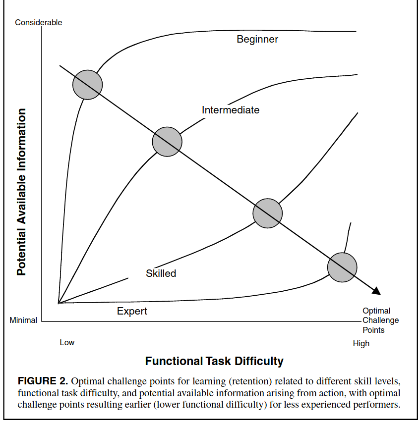
The CPF suggests that as one's skill increase in a task, learning is optimized when task difficulty is increased as well. This relationship is explained by higher ability to utilize additional information for learning when task skill increases, and additional information improves learning. In contrast, extra information presented during to someone with a low skill level, and thus low ability to utilize information, impedes the learning process by overwhelming the cognitive resources available during learning.
A key idea is that increasing task difficulty is associated with increasing information available to the learner for the following reasons:
Model someone being highly skilled in a motor task with the expected success of his movement plan in the task being very high. In this case, a negative result would yield more information about the learner's internal model. In contrast, a positive result does not provide much useful information.
When task difficulty is low, he would expect success, therefore learning is minimal.
When task difficulty is high, likelihood for negative result is higher, therefore the potential information available to the learner is higher. More potential information implies more learning is possible.
A related way to see it is that "practice leads to redundancy, less uncertainty, and, hence, to reduced information". The more that practice leads to better expectations, the less information there will be to process.
Therefore in this framework, factors that contribute to motor learning can be easily evaluated to predict its effects on skill performance and learning. Factors influencing learning include:
Task difficulty: note this can be divided into the inherent or nominal difficulty, and functional difficulty. A nominally difficult task can be made to have less functional difficult task by introducing helpful feedback, for example.
Practice schedule (changes the functional difficulty): blocked, random, randomized block. Random practice schedule increases the functional difficulty wrt blocked practice schedule due to contextual interference.
Feedback (also known as knowlege of result - KR) and feedback schedule:
More frequent feedback lowers functional difficulty
Random feedback schedule increases functional difficulty, compared to blocked schedule.
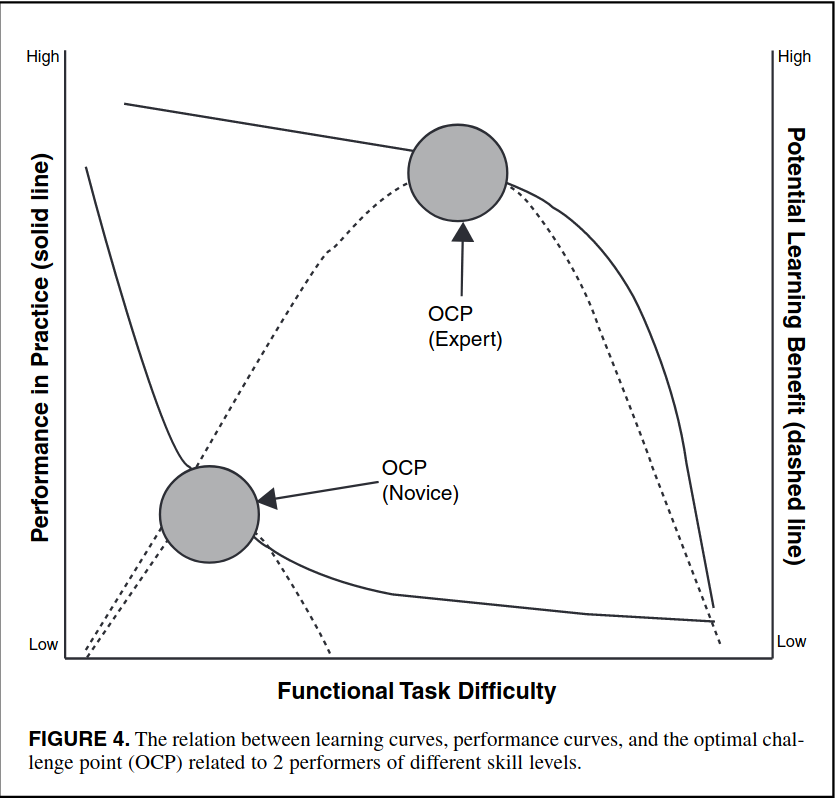
This framework also predict optimal challenge point, as a function of task difficulty and skill level, during which learning (or utilizable potential information availability) is maximized.
Details
Definitions
Nominal task difficulty: The difficulty of a particular task within the constraints of an experimental protocol. The nomianl difficulty of a task is considered to reflect a constant amount of task difficulty, regardless of who is performing the task and under what conditions it is being performed. This makes the most sense in comparison with other skills, for example, kicking a ball 50 meters has more nominal difficulty than kicking it 1m, and less than kicking it 100 meters.
Functional task difficulty: How challenging the task is relative to the skill level of the individual performing the task and to the conditions under which it is being performed. Ex: kicking a ball 50 meters has the same nominal difficulty to amateur and pro, but different functional difficulty (i.e. success rate).
Practically, nominal task difficulty is probably not important to think about.
Assumptions
Learning is a problem-solving process in which the goal of an action represents the problem to be solved and the evolution of a movement configuration represents the performer's attempt to solve the problem.
Source of information available during and after each attempt is remembered and form the basis for learning, resulting in improvement skill -- this is practice.
Two sources of information are criticle for learning: the action plan (known to a priori to the learner), and feedback (obtained during or after).
Optimal challenge point
In CPF, learning is directly related to the information available and interpretable in a performance instance, which, in turn is tied to the functional difficulty of the task. The central thesis is then:
Information represents a challenge to the performer and that when information is present, there is potential to learn from it
Subsequent corollaries are:
Learning cannot occur in the absence of information
Learning will be impeded in the presence of too much information (too much challenge, cognitive overload).
Learning achievement depends on an optimal amount of information, which differs as a function of the skill level of the individaul.
Therefore, the factors contributing to functional task difficulty interact to dictate the optimal amount of interpretable information, and thus the potential for learning.
Corollary 2 derives from the observation that if information is to result in learning, it must be interpretable. The total amount of information one can interpret is goverend by one's information-processing capabilities, which changes with practice.
As skill improves, the expectation for performance becomes more challenging. So to generate a challenge for learning, one must obtain increased information, which can arise only from an increase in the functional task difficulty. Luckily, both information-processing capability and skill level increases with practice.
Predictions of CPF
Practice variables that influence action planning information via contextual interference (most often random practice schedule is proxy for contextual interference):
For tasks with differing levels of nominal difficulty, the advantage of random practice (vs. blocked practice) for learning will be largest for tasks of lowest nominal difficulty and smallest for tasks of highest nominal difficulty.
For individuals with differing skill levels, low levels of CI will be better for beginning skill levels and higher levels of CI will be better for more highly skilled individuals (via increasing functional difficulty).
Modeled information (i.e. examples and prior demos) decrease functional difficulty.
Practice variables that influence feedback information (knowledge of result, among other things):
For tasks of high nominal difficulty, more frequent or immediate presentation of KR, or both, will yield the largest learning effect. For tasks of low nominal difficulty, less frequent or immediate presentation of KR, or both, will yield the largest learning effect
For tasks about which multiple sources of augmented information can be provided, the schedule of presenting the information will influence learning. For tasks of low nominal difficulty, a random schedule of augmented feedback presentation will facilitate learning as compared with a blocked presentation. For tasks high in nominal difficulty, a blocked presentation will produce better learning than a random schedule.
How to apply?
Athletic skills is perhaps the obvious example: boxers practice individual punches first (blocked practice schedule, frequent feedback, easy), before mixing it in combinations and sparring.(random practice schedule, summary/infrequent feedback, difficult).
Tutorials: Introduce concept one at a time (less information and less difficulty)
A practice schedule or learning plan can be very important in skills and knowledge acquisition, thus the saying "perfect practice makes perfect". I first heard about this work on Andrew Huberman's podcast on goal setting. The results here are significant, offering insights into both training ML algorithms, as well as biological learners. Furthermore, the analysis techniques are elegant, definitely brushed off some rust here!
Summary
Examine the role of the difficulty of training on the rate of learning.
Theoretical result derived for learning algorithms relying on some form of gradient descent, in the context of binary classification.
Note that gradient descent here is defined as where "parameters of the model are adjusted based on feedback in such a way as to reduce the average error rate over time". This is pretty general, and both reinforcement learning, stochastic gradient descent, and LMS filtering can be seen as special cases.
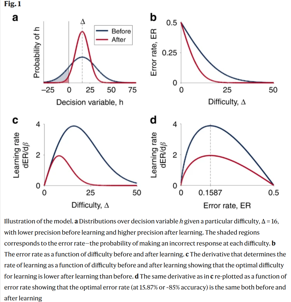
Results show under Gaussian noise distributions, the optimal error rate for training is around 15.87%, or conversely, the optimal training accuracy is about 85%.
The noise distribution profile is assumed to be fixed, i.e. the noise distribution won't change from Gaussian to Poisson.
The 15.87% is derived from the value of normal CDF with value of -1.
Under different fixed noise distributions, this optimal value can change.
Training according to fixed error rate yields exponentially faster improvement in precision (proportional to accuracy), compared to fixed difficulty. vs. .
Theoretical results validated in simulations for perceptrons, 2-layer NN on MNIST dataset, and Law and Gold model of perceptual learning (neurons in MT area making decision about the moving direction of dots with different coherence level, using reinforcement learning rules).
Some background
The problem of optimal error rate pops up in many domains:
Curriculum learning, or self-paced learning in ML.
Level design in video games
Teaching curriculum in education
In education and game design, empirically we know that people are more engaged when the tasks being presented aren't too easy, and just slightly more difficult. Some call this the optimal conditions for "flow state".
Problem formulation
The problem formulation is fairly straight-forward, as the case of binary classification and Gaussian noise.
Agent make decision, represented by a decision variable , computed as , where is the stimulus, and are the parameters of whatever learning algorithm.
The decision variable is a noisy representation of the true label : , where .
If the decision boundary is set at (see Figure 1A), such that chose A when , B when and randomly otherwise, then the decision noise leads to error rate of: \[ER = \int_{-\infty}^{0} p(h|\Delta,\sigma)dh=F(-\Delta/\sigma)=F(-\beta\Delta)\].
p() is Gaussian distribution
F() is Gaussian CDF
is precision, and essentially measures how "peaky" the decision variable distribution is. This can be thought of as the (inverse) accuracy or "skill" of the agent.
So, the error decreases with both agent skill ( ) and ease of problem ( ).
Learning is essentially an optimization problem, to change in order to minimize . This can be formulated as a general gradient descent problem: \[\frac{d\phi}{dt}=-\eta\nabla_\phi ER\].
This gradient can be written as . And we want to find the optimal difficulty that maximizes .
turns out to be , which gives optimal error rate .
This is nice, the difficulty level should be proportional to the skill level.
Simulations
Validation of this theory boils down to the following elements:
How to quantify problem/stimulus difficulty ?
How to select problem with the desired difficulty?
How to adjust target difficulty level to maintain the desired error rate?
How to measure error rate ?
How to measure skill level?
Application to perceptron:
A fully trained teacher perceptron network's weights are used to calculate the difficulty. The difficulty of a sample is equal to its distance from the decision boundary (higher is less difficult).
Skill level of the network is , where is the angle between the learner perceptron's weight vector and the teacher perceptron's weight vector.
Error rate is approximately Gaussian and can be determined from the weight vectors of the teacher and learner perceptrons, and the sample vectors.
Application to two-layer NN:
Trained teacher network. The absolute value of the teacher network's sigmoid output is the difficulty of a stimulus.
Error rate is the accuracy over the past 50 trials (not batch training).
Skill level is the final performance over the entire MNIST dataset.
Difficulty level is updated with value proportional to the current and target accuracy level.
Appliation to Law and Gold model:
Simulated update rule of 7200 MT neurons according to the orignal reinforcement model.
Coherence adjusted to hit target accuracy level: implicitly measure difficulty level
Accuracy/error rate is from past running average
Final skill level is from applying ensemble on different coherence level stimulus (disabling learning) and fitting logistic regression.
Implications
Optimal rate is dependent on task (binary vs. multi-class), and noise distribution.
Batch learning makes things more tricky -- depending on agent learning rate.
Multi-class may require finer grained evaluation of difficulty and problem preseentation (i.e. misclassifying 1v2, or 2v3).
Not all models follow this framework, e.g. Bayesian learner with perfect memory does not care about example presentation order.
Can be a good model for optimal use of attention for learning -- suppose exerting attention changes the precision , then the benefits of exerting attention is maximized during optimal error rate.
Continuing on my quest to have the best unifying intuition about linear algebra, I came across the excellent series Essence of Linear Algebra on YouTube by 3Blue1Brown.
This series really expanded on the intuition behind the fundamental concepts of Linear Algebra by illustrating them geometrically. I have vaguely arrived at the same sort of intuition through thinking about them before, but never this explicitly. My notes are here.
Vectors can be visualized geometrically as arrows in 1-D, 2-D, 3-D, ..., n-D coordinate system, and can also be represented as a list of numbers (where the numbers represent the coordinate values).
The geometric interpretation here is important to build interpretation and can later be gneralized to more abstract vector spaces.
Vectors (arrows, and list of numbers) can form linear combinations, which can involve multiplication by scalars and addition of vectors. Geometrically, multiplication by scalar is equivlaent to scaling the length of a vector by that factor. Vector addition means putting vectors tail to head and find the resulting vector.
Any vectors in 2D space, for example, can be described by linear combinations of a set of basis vectors.
In other words, 2D space are spanned by a set of basis vectors. Usually, the basis vectors are chose to be and in 2-D, representing the unit and vectors.
As a corollary, if a 3-by-3 matrix has linearly-dependent columns, that means its columns does not span the entire 3D-space (spans a plane or a line instead).
Multiplication of a 2-by-1 vector by an 2-by-2 matrix to yield a new 2-by-1 vector : can be thought of as a linear transformation. In fact, this multiplication can be thought of as transforming the original 2-D coordinate system into a new one, with the caveat the grid lines still have to remain parallel after the transformation (think about a grid getting sheared or rotated).
Specifically, assume the original vector is written with basis vectors and , the columns of can be thought of where and land in the transformed coordinate system.
Therefore, the matrix-vector multiplication then has the geometric meaning of representing the original vector as linear combination of the original basis vectors and , finding where they map to in the transformed space (indicated by matrix ), and then yielding as the same linear combination of the transformed basis vectors.
This is a very powerful idea -- the specific operation of matrix-vector multiplication makes clear sense under this context.
If a matrix represents a transformation of the coordinate system (e.g. shear, rotation), then multiplication of matrices represent sequences of transformations. For example can represent first shear the coordinate system () then rotate the resulting coordinate system ().
This also makes it obvious why matrix multiplication is NOT commutative. Shearing a rotated coordinate system can have different end result as rotating a sheared coordinate system.
Inverse of a matrix then represents performing the reverse coordinate system transformation, such that represents net-zero transformation of the original coordinate system, which is exactly represented by the identity matrix.
This is a really cool idea. In many statistics formulas, there will be a condition that reads like "assuming is positive-definite, we multiply by ". Positive-definite relates to positive determinants. This gave me the sense that determinant represents a matrix analog of real number's magnitude. But then what does a negative determinant mean?
In the 2D case, if a matrix represents a transformation of the coordinate system, the determinant then represents the area in the transformed coordinate system of a unit area in the original system. Imagine a unit square being stretched, what is the area of the resulting shape -- that is the value of the determinant.
Negative determinant would mean a change in the orientation of the resulting shape. Imagine a linear transformation as performing operations to a piece of paper (parallel lines on the paper are preserved through the operations). Matrix with determinant of -1 would correspond to operations that involve flipping the paper. is originally 90-degrees clockwise from , after flipping the paper (x-y plane), is now 90-degrees counter clockwise from .
In 3D, determinant then measures the scaling a volume, and negative determinant represent transformations that does not preserve the handed-ness of the basis vectors (i.e. right-hand rule).
If negative determinant represent flipping a 2D paper, then 0 determinant would mean a unit-area becoming zero. Similarly, in 3D, 0 determinant would mean a unit-volume becoming zero. What shape has 0 volume? A plane, a line, and a point. What shape has 0 area? A line and a point.
So if , then we know transforms maps vectors into a lower-dimensional space! And that is why positive-definiteness is important, it means a transformation perserves the dimension of the data!
From this intuition, the computation of determinant also makes a bit more sense (at least in the 2D case).
This chapter combines the geometric intuition from before and solving systems of linear equations to explain inverse matrices, column space, and null space.
Inverse matrices
Solving system of linear equations in the form of (where A=3-by-3, x and v are 3-by-1 vectors) can be thought of as what vector in 3-D space, after transformation represented by , become the vector ?
In this nominal case where , there exists an inverse that represents the inverse transformation represented by , and thus can be solved by multiplying on both sides of the equation.
Intuitively this makes sense -- to get the vector pre-transformation, we simply reverse the transformation.
Now suppose , this means maps a 3-D vector onto a lower-dimensional space, which can be a plane, a line, or even a point. In this case, no inverse exists, because how can you transform these lower-dimensional constructs into 3D space? (Note that in most textbooks, the justification of exists only when is not zero is made on the basis of Gauss-Jordan form, which is not intuitive at all).
Column Space and Null Space
So in the nominal case, each vector in 3D is mapped to a different one in 3D space. Therefore the set of all possible 's span the entire 3D space. Therefore the 3D space is the column space of the matrix . The rank of in this case is 3, because the column space is 3-dimensional.
The set of vectors that after transformation by yield the 0-vector are called the null space of the matrix .
In cases where , the columns of must be linearly dependent, this means its column space is not 3-dimensional, and therefore its rank is less than 3 (and therefore is rank-deficient and not full-rank for a 3-by-3 matrix).
If this rank-deficient maps onto a plane, then its column space has rank 2. Onto a line -- rank 1; Onto a point -- rank 0. For a 3-by-3 matrix, 3 minus the rank of the column space is the rank or dimension of the null-space.
Geometrically, this means if a transformation compresses a cube into a plane, then an entire line of points are mapped onto the origin of the resulting plane (imagine a vertical compression of a cube, the entire z-axis is mapped onto the origin and is therefore the null space of this transformation). Similarly, if a cube is compressed into a line, then an entire plane of points are mapped onto the origin of the resulting number line.
Left and Right Inverse
Technically, the inverse normally talked about refers to the left inverse (). And the full-rank matrices for which left inverse exist perform a one-to-one transformation of vectors (injective) -- each unique vector is mapped onto at most one vector.
For matrices with more columns than rows, the situation is a bit different. Using our intuition from before treating the columns of matrix as mapping of the original basis vectors into a new coordinate system, consider the matrix mapping a 3D vector. This matrix maps the basis vectors , and onto an entire plane, respectively. Therefore each transformed vector can have multiple corresponding vectors in the original 3D space (therefore is called surjective).
Consequently, if is 2-by-3, there exists a 3-by-2 right-inverse matrix such that , but here is 2-by-2. Geometrically, this is saying if we transform a 2D vector onto 3-space (), we can recover this 2D vector by another transformation (). Thus right-inverse deal with transformations involving dimensional changes.
These explanations, in my opinion, are much more intuitive and easy to remember than the rules and diagram taught in all of the linear algebra courses I have ever taken, including 18.06.
This one is pretty interesting. Dot product represents projection. At the same time, we can think of dot product in 2D, as a matrix-vector multiplication . Here we can think of the "matrix" as a transformation of the basis 2D basis vectors and onto vectors on the number line. Therefore dot-product represents a 2D-to-1D transformation.
This is the idea of vector-transformation duality. Each n-dimensional vector's transpose represents an N-to-1 dimensional linear transformation.
This one is also not too insightful, perhaps because cross product's definition as a vector was strongly motivated by physics.
Cross-product of two 2D vectors and yield a third vector perpendicular to both (together obeying right-hand rule) with magnitude equal to the area of the parallelogram formed by the and . Thinking back, cross-product formula involves calculating a type of determinant -- which makes sense in terms of the area interpretation of the determinant.
Then the triple product represents the volume of the parallelpiped formed by , , and .
This one basically explains the triple product by interpreting the dot-product operation () by the cross-product () as finding a 3D-to-1D linear transformation.
This also follows from the idea that a matrix represents mapping of the individual vectors of a coordinate system.
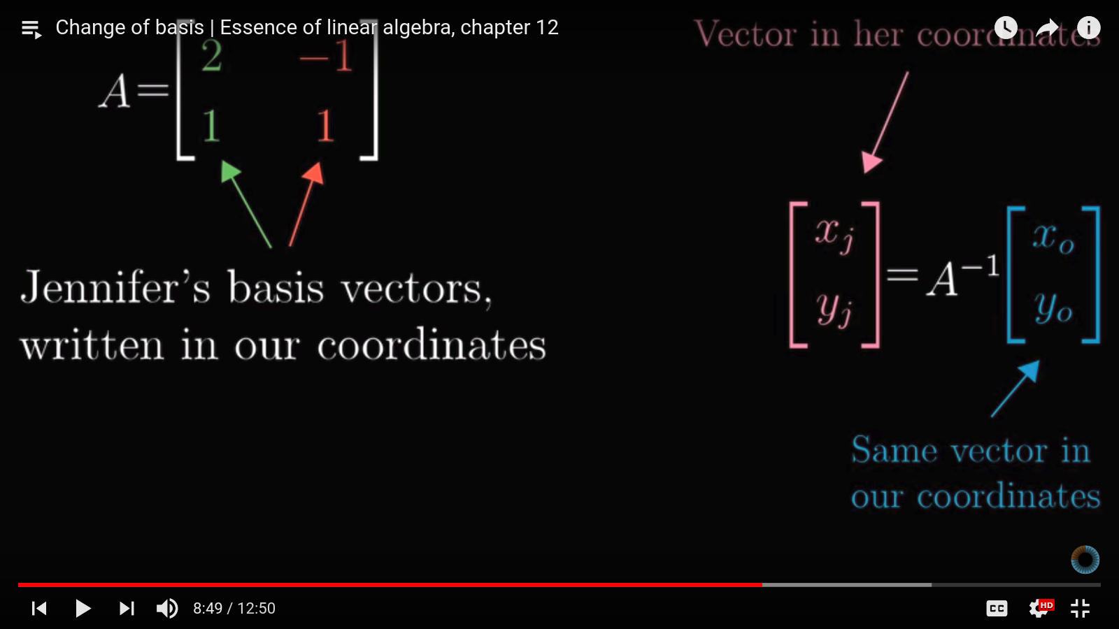
The idea is that coordinate systems are entirely arbitrary. We are used to having and as our basis vectors, but they can be a different set entirely. Suppose Jennifer has different basis vectors and , how do we represent a vector in our coordinate system in Jennifer's coordinate system?
This is done by a change of basis -- by multiplying by a matrix whose columns are Jennifer's basis vectors. This is yet another application of matrix-vector product.
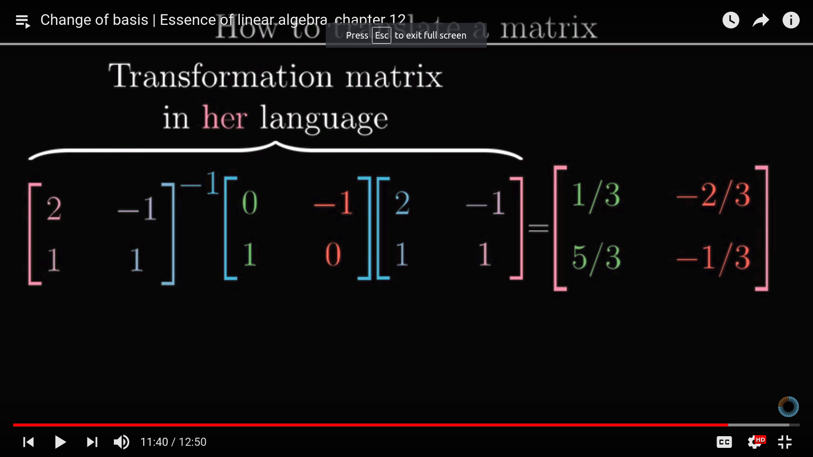
Change of basis can also be applied to translate linear transformations. For example, suppose we want to rotate the vector in Jennifer's coordinate system by 90 degrees and want to find out the result in Jennifer's coordinate system. It may be tedious to figure out what the 90-degree transformation matrix is in Jennifer's coordinate system, but it is easily found in our system ().
So we can achieve this easily by first transforming into our coordinate system by multiplying it by the mapping between Jennfier and our coordinate system. Then apply the 90-degree transformation matrix, then apply the inverse transformation to get back the resulting vector in Jennifer's system.
This is a powerful idea and relates closely to eigenvectors, PCA, and SVD. SVD especially represents a matrix by a series of coordinate transformations (rotation, scaling and rotation).
This is motivated by the problem , where are the eigenvectors, and are the eigenvalues of the matrix (nominally, is a square matrix, otherwise we use SVD, but that is beside the point).
The eigenvectors are vectors that, after transformation by , still point at the same directions as before. A unit vectors before after the transformation may have different length while pointing to the same direction, the change in length is described by the eigenvalue. A negative eigenvalue means the eigenvectors have reversed where it points to after the transformation.
The imagery is suppose we have a square piece of paper/mesh, we pull at the top right and bottom left corners to shear it. A line connecting this two corners will still have the same orientation, though have longer length. Thus this line is an eigenvector, and the eigenvalue will be positive.
However, if a matrix represents rotation, then the determinant will be 0, and the eigenvalues will be imaginary. Imaginary eigenvalues means that a rotation is involved in the transformation.
This lesson extrapolate vectors, normally thought of as arrows in 1- to 3-D space and corresponding list of numbers, to any construct that obey the axioms of vector space. Essentially the members of a vector space follow the rule of linear combination (or linearity).
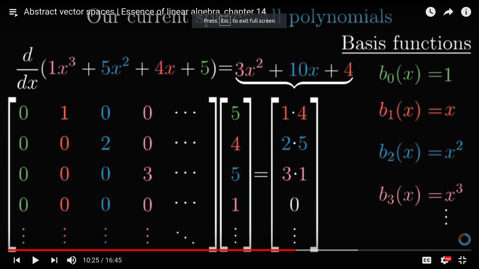
An immediate generalization is thinking of functions as infinite-dimensional vectors (we can add scalar multiples of functions together and the result obey the linearity rule). We can further define linear transformations on these functions, similarly to how matrices are defined on geometric vector spaces.
An example of linear transformation on function is derivative.
This insight is pretty cool and really ties a lot of math and physics concepts together (ex. modeling wavefunctions as vectors in quantum mechanics, eigen-functions as analogs of eigen-vectors).
Writing my dissertation I chose to use Latex because it makes everything looks good, I can stay in Vim, type math easily, and don't have to deal with an actual Word-like processor's abysmal load speed when I'm writing 100+ pages. At the same time, some things that should be very easy took forever to figure out.
Problem
In addition to the bibliography of the actual dissertation chapters itself, I need to append a list of my own publications in the biography section (last "chapter" of the entire document), formatted like a proper bibliography section. Why biography? So future readers would known which John Smith you are, of course!
This is difficult for several reasons.
The top level dissertation.tex is something like
\documentclass[]{dissertation}% Package setup, blabla\begin{document}\tableofcontents\listoftables\listoffigures\include{{./Chapter1/ch1.tex}}% Separate tex-file and folder for other chapters\include{{./Chapter2/ch2.tex}}% \include for all the chapters% Now in the end insert a single bibliography for all the chapters\bibliographystyle{myStyle}% uses style defined in myStyle.bst\addcontentsline{toc}{chapter}{Bibliography}% Add it as a section in table of content\bibliography{dissertation_bib_file}% link to the bib file \include{{./Biography/biography}}\end{document}
If I were using word, I might just copy and paste some formatted lines to the end of the page and call it a day. But since I am a serious academic and want to do this the right away...it poses a slight struggle. I need to make bibtex format my publications and insert it at the end during the compile process. My requirements:
I don't want the publication list to start with a "Reference" section heading like typical \bibliography{bib_file} commands produce.
I want the items in the publication list to be in reverse chronological order, from most recent to least.
I want to allow my publication list to be separate from the main bibliography section -- an item can appear in both places, but they should have the same numbering.
Approach 1
Created a separate bibtex file mypub.bib, then inserted the following lines in biography.tex:
\nocite{*}% needed to show all the items in the bib-file. % Otherwise only those called with \cite{}\bibliographystyle{myStyle}% uses style defined in myStyle.bst\bibliography{mypub}% link to second bib file
I don't remember the exact behavior, but it either
Gives error, pdflatex tells me I can't call \bibliography in multiple places. Or
Insert the entire dissertation's bibliography after the biography section.
Neither is desirable.
Approach 2
Searching this problem online, you run across people wanting to
Have a bibliography section for each chapter
Divide biblography into nonoverlapping sets, such as journals, conference proceedings, etc.
% preamble stuff\usepackage{multibib}\newcites{pub}{headingTobeRemoved}% create a new bib part called 'pub' with heading 'headingTobeRemoved`\begin{document}% all the chapter includes% Now in the end insert a single bibliography for all the chapters\bibliographystyle{myStyle}% uses style defined in myStyle.bst\addcontentsline{toc}{chapter}{Bibliography}% Add it as a section in table of content\bibliography{dissertation_bib_file}% link to the bib file \include{{./Biography/biography}}\end{document}
Really important in the second reference section to use \nocitepub, \bibliographystylepub, and \bibliographypub such that it matches the name of the \newcites group.
where dissertation.aux contains the bib-entries to use in the main document's reference section, and pub.aux contains that for the biography's publication list.
This got me a list at the end of the biography chapter. But it starts with a big heading, it's not in reverse chronological order but alphabetical (because myStyle.bst organizes bibs that way), and the numbering is not diea. For example, one of the item in mypub.bib is also in dissertation_bib_file.bib, and their numbering is the same in both places such that in the publication list, I have item ordering like 1, 2, 120, 37, 5...
No good.
Removing Header
In biography.tex, included the following suggest by SO post
Internally bibliography implements its header as a section or chapter header, so the \renewcommand suppresses it.
Get rid of weird ordering
This took the longest time and I could not find a satisfactory solution. Using
\usepackage[resetlabels]{multibib}
did not help. Nobody seems to even have this problem...so I gave up and just made the items use bullets instead. In biography.tex:
Blablabla memememeem
\renewcommand{\chapter}[2]{}% ---- next three lines make bullets happen ---\makeatletter\renewcommand\@biblabel[1]{\textbullet}% Can put any desired symbol in the braces actually\makeatother% -----------------\nocitepub{*}\bibliographystylepub{myStyle}\bibliographypub{mypub}
Reverse chronological order
This one is very tricky, and requires modifying the actual myStyle.bst file. This SO post gives a good idea of how these bst-files work...they really have a weird syntax. Basically, in every bst file, a bunch of functions are defined and used to format individual reference entries from the bibtex entry, then these entries are sorted and inserted into the final file. The function that likely needs to be changed in all bst-files is the PRESORT function.
plainyr-rev.bst provides a working example of ordering reference entries in reverse chronological order. I decided to use jasa.bst, from Journal of American Statistical Association. The following are the changes needed:
%%%%%%% Extra added functions %%%%%%%%%%%%%%%% From plainyr_rev.bst
FUNCTION {sort.format.month}{ 't :=
t #1 #3 substring$ "Jan" =
t #1 #3 substring$ "jan" =
or
{ "12" }{ t #1 #3 substring$ "Feb" =
t #1 #3 substring$ "feb" =
or
{ "11" }{ t #1 #3 substring$ "Mar" =
t #1 #3 substring$ "mar" =
or
{ "10" }{ t #1 #3 substring$ "Apr" =
t #1 #3 substring$ "apr" =
or
{ "09" }{ t #1 #3 substring$ "May" =
t #1 #3 substring$ "may" =
or
{ "08" }{ t #1 #3 substring$ "Jun" =
t #1 #3 substring$ "jun" =
or
{ "07" }{ t #1 #3 substring$ "Jul" =
t #1 #3 substring$ "jul" =
or
{ "06" }{ t #1 #3 substring$ "Aug" =
t #1 #3 substring$ "aug" =
or
{ "05" }{ t #1 #3 substring$ "Sep" =
t #1 #3 substring$ "sep" =
or
{ "04" }{ t #1 #3 substring$ "Oct" =
t #1 #3 substring$ "oct" =
or
{ "03" }{ t #1 #3 substring$ "Nov" =
t #1 #3 substring$ "nov" =
or
{ "02" }{ t #1 #3 substring$ "Dec" =
t #1 #3 substring$ "dec" =
or
{ "01" }{ "13" }% No month specified
if$
}
if$}
if$
}
if$}
if$
}
if$}
if$
}
if$}
if$
}
if$}
if$
}
if$}% Original jasa's presort function%FUNCTION {presort}%{ calc.label% label sortify% " "% *% type$ "book" =% type$ "inbook" =% or% 'author.editor.sort% { type$ "proceedings" =% 'editor.sort% 'author.sort% if$% }% if$% #1 entry.max$ substring$% 'sort.label :=% sort.label% *% " "% *% title field.or.null% sort.format.title% *% #1 entry.max$ substring$% 'sort.key$ :=%}% New one from plainyr_rev.bst
FUNCTION {presort}{% sort by reverse year
reverse.year
" "
*
month field.or.null
sort.format.month
*
" "
*
author field.or.null
sort.format.names
*
" "
*
title field.or.null
sort.format.title
*
% cite key for definitive disambiguation
cite$
*
% limit to maximum sort key length
#1 entry.max$ substring$
'sort.key$ :=
}
ITERATE {presort}% Bunch of other stuff% ...
EXECUTE {initialize.extra.label.stuff}%ITERATE {forward.pass} % <--- comment out this step to avoid the % year numbers in the reverse-chronological% entry to have letters following the year numbers
REVERSE {reverse.pass}%FUNCTION {bib.sort.order}%{ sort.label% " "% *% year field.or.null sortify% *% " "% *% title field.or.null% sort.format.title% *% #1 entry.max$ substring$% 'sort.key$ :=%}%ITERATE {bib.sort.order}
SORT % Now things will sort as desired
Extra: Make my name bold
Might as well make things nicer and make my name bold in all the entries in my publication list. This post has many good approaches. Considering I'm likely only to have to do this once (or very infrequently), I decided to simply alter the mypub.bib file.
Suppose your name is John A. Smith. Depending on the reference style and the specific bibtex entry, this might become something like Smith, J. A., Smith, John A., Smith, John, or Smith, J..
In bibtex, the author line may be something like:
% variation 1
author = {Smith, John and Doe, Jane}% variation 2
author = {Smith, John A. and Doe, Jane}
Apparently the bst files simply goes through these lines, strsplit based on keyword "and", and take the last name and first name field and contatenate them together. And if only initial is needed, take the first letter of the first name. So, we can simply make the correct fields bold:
There are some important signal processing points I keep having to re-derive, is rarely mentioned in the textbooks, and buried deep in the math.
What is the physical significance of negative frequencies?
FFT of real signals usually have both positive and negative frequencies in their spectrum. In feedback analysis, we simply ignore the negative frequencies and look at the positive part.
A good illustration of what is actually happening is below:
The spiral can spin counter-clockwise or clock-wise, corresponding to positive or negative frequency. From the formula of Fourier Transform , we can see the frequency spectrum of a signal actually correspond to that of the spiral. Therefore both and are the sum of two complex exponentials. This is in fact true for all real, measurable signals.
In contrast, in Hilbert transform, the analytic signal has single-sided spectrum, which is not physically realizable. However, it allows us to derive the instantaneous amplitude and frequency of the actual time-domain signal .
Why is a linear phase response desirable for a system?
I always get tripped up by the language. I used to see a phase-response that is not flat and think the different frequencies have different phase lag, therefore they are going to combine at the output and the signal is going to be distorted.
The first part of that thought is correct, but the implication is different. 90-degrees phase-lag for a low-frequency signal is much longer in the time-domain as 90-degrees phase-lag for a high-frequency signal. Therefore, if all frequencies need to be delayed the same amount of time, the phase-lag need to be different.
In math, suppose an input signal is filtered to output given by , which is a pure delay by . This can then be written as , where is the phase response of the system, and the phase becomes more negative for larger frequencies.
And this is why linear phase response is desirable for a system.
The success of deep neural network techniques have been so great leading to the hype general intelligence can be achieved soon. I had my doubts, mostly based on the amount of data needed compared to examples needed for people to learn, but also on possible biological mechanisms that could implement backpropagation that is central to artificial neural networks. More neuroscience discoverys are needed.
The great Hinton made a big splash with the capsule theory. Marblestone et al., 2016 had many speculations on how backprop could be approximated by various mechanisms.
Some cool recent results:
Delahunt 2018: Biological mechanisms for learning, a computational model of olfactory learning in the Manduca sexta Moth, with applications to neural nets. TR interview
The insect olfactory system [...] process olfactory stimuli through a cascade of networks where large dimension shifts occur from stage to stage and where sparsity and randomoness play a critical role in coding.
Notably, a transition from encoding of stimulus from a low-dimensional parameter space to one in a high-dimensional parameter space occur, not too common in ANN architectures. Reminds me of the kernel transformations.
Learning is partly enabled by a neuromodulatory reward mechnaism of octopamine stimulation of the antennal lobe, whose increased activity induces rewiring of the mushroom body through Hebbian plasticity. Enforced sparsity in the MB focuses Hebbian growth on neurons that are the most important for the representation of the learned odor.
Potential augment to backprop at least. Also, octopamine opens new transmitting channels for wiring expanding the solution space.
Akrami 2018: PPC represents sensory history and mediates its effects on behavior. Shows PPC's role in the representation and ues of prior stimulus information. Cool experiments showing Bayesian aspect of the brain. As much as I dislike Bayesian techniques..
Nikbakht 2018 Supralinear and supramodal integration of visual and tactile signals in rats: psychophysics and neuronal mechanisms.
. Rats combine vision and touch to distinguish two grating orientation categories.
. Performance with vision and touch together reveals synergy between the two channels.
. PPC neuronal responses are invariant to modality.
. PPC neurons carry information about object orientation and the rat's categorization.
Linear model is a crazy big subject, dividing into:
LM (linear models) -- this includes regressions by ordinary least squares (OLS), as well as all analysis of variance methods (ANOVA, ANCOVA, MANOVA). Assumes normal distribution of the dependent variable.
GLM (generalized linear models) -- linear predictor and dependent variable related via link functions (poisson, logistic regressions fall into this category).
ANOVA and friends (and their GLM analogs) in GLM and LM are achieved through the introduction of indicator variables representing "factor levels".
GLMM (generalized linear mixed models) -- Extension of GLMs to allow response variables from different distributions. Mixed refers to both fixed and random effects.
Repeated measures is when the same set of subjects, divided into different treatment groups, are measured over time. It would be silly to treat all of the measurements as independent. Advantage is there is less variance bebetween measurements taken on the same subject. Consequently, a repeated measures design allow for same statistical power with less subjects (compared to another design where N different subjects are measured at the different time points and treating all these measurements as independent).
This can be achieved through:
MANOVA approach - The measurements of all subjects at a given time is a length-n vector and becomes the dependent variable of our MANOVA.
GLMM - controls for non-independence among the repeated observations for each individual by adding one or more random effects for individuals to the model.
Variance, Deviance, Sum of Squares (SS), Clustering, and PCA
In LM and ANOVA-based methods, we try to divide the total sum of squares (measuring the response deviation of all data points from the grand mean) into components that can be explained by the predictor variables. A good mental picture to have is:
.
Don't mind that it is in 2D, it actually illustrates the generalization of ANOVA into MANOVA. In ANOVA, response values are distributed along a line, in MANOVA, response values are distributed in n-dimensional space. As we see here, the within-group sum of squares (SSW) is the sum of squared distances from individual points to their group centroid. The among-group sum of squares (SSA) is the sum of squared distances from group centroids to the overall centroid. In ANOVA methods, a predictor's effect is significant if the F-test statistic, proportional to the ratio of SSA and SSW hits the critical value.
The analogous method is the analysis of deviance in GLM methods, where we are comparing likelihood ratios instead of SS ratios. Still a bitch though.
This framework of comparing dissimilarity or distance is very useful, especially in constructing randomization-based permutation tests. The excellent paper by Anderson 2001 describes how to use this framework to derive a permutation-based non-parametric MANOVA test. This was implemented in MATLAB in the Fathom toolbox.
A key insight is as shown in the following picture
The sum of squared distances from individual points to their centroid is equal to the sum of squared distances divided by the number of points. Why is this important? Anderson explains:
In the case of an analysis based on Euclidean distances, the average for each variable across the observations within a group constitutes the measure of central location for the group in Euclidean space, called a centroid. For many distance measures, however, the calculation of a central location may be problematic. For example, in the case of the semimetric Bray–Curtis measure, a simple average across replicates does not correspond to the ‘central location’ in multivariate Bray–Curtis space. An appropriate measure of central location on the basis of Bray–Curtis distances cannot be calculated easily directly from the data. This is why additive partitioning (in terms of ‘average’ differences among groups) has not been previously achieved using Bray–Curtis (or other semimetric) distances. However, the relationship shown in Fig. 2 can be applied to achieve the partitioning directly from interpoint distances.
Brilliant! Now we can use any metric -- SS, Deviance, absolute value, to run all sorts of tests. Note now we see how linear models are similar to clustering methods, but supervised (i.e. we define the number of clusters by the number of predictors).
Projecting data to subspace to maximize the projected data's variance. This is the traditional and easiest approach to understand.
A complementary formulation to the previous one is projecting data to subspace to mimimize the projection error. This is basically linear regression by OLS. There is even a stackexchange question on it.
Probabilistic PCA. In this approach, PCA is described as the maximum likelihood solution of a probabilistic latent variable model. In this generative view, the data is described as samples drawn according to
This is a pretty mind blowing formulation which would link PCA, traditionally a dimensionality reduction technique, with factor analysis that describe latent variables. There is a big discussion on stackexchange on this generative view of PCA.
Bayesian PCA. Bishop is a huge Bayesian lover, so of course he talks about making PCA Bayesian. A cool advantages is automatic selection of principal components by giving the vectors of a prior which is then shrunk during the EM procedures. Another cool thing about PPCA/Bayesian PCA is the iterative procedure allows estimating the top principal components without computing the entire covariance matrix/eigenvalue decomposition.
Factor Analysis. This is treated as a generalization of PPCA, where instead of , we have
where is still a diagonal matrix, but the individual variance values are not the same. This has the following consequences of using PCA vs. FA, quoting amoeba,
As the dimensionality n increase, the diagonal [of sampling covariance matrix] becomes in a way less and less important because there are only n elements on the diagonal and O(n^2) elements off the diagonal. As a result, for the large n there is usually not much of a difference between PCA and FA at all [...] For small n they can indeed differ a lot.
One common misconception among neuroscientists (and me, until a short while ago) is to use conventional non-parametric tests such as WIlcoxon, Mann-Whitney, Kruskal-Wallis, etc as a cure-all for violation of assumptions in the parametric tests. However, these tests simply replace the actual response values by their ranks, then proceed with calculating sum of squares, and using a test statistic instead of an F-test.
The Chi-squared distribution of the test statistic is based on the assumption that ranked data for each treatment level are samples drawn from distributions that differe only in location (e.g. mean or median). The underlying distributions are assumed to have the same shape (i.e. all other moments of the distributions-- the variance, skewness, and so on -- are identical). These assumptions about nonparamteric tests are often not appreciated, and ecologists often assume that such tests are distribution-free).
Hence the motivation for many permutation based tests, which Anderson notes can detect both variance and location differences (but not correlation difference). Traditional parametric tests, on the other hand, are also sensitive to correlation and dispersion differences (hence why everyone loves them).
 .
.