
LMS is the second stage of processing in RHA-headstage’s signal chain, after AGC. It aims to estimate the noise common to all electrodes and subtract that noise from each channel.
Adaptive Filtering Theory
Chapter 12 on Adaptive Interference Cancelling in Adaptive Signal Processing by Bernard Widrow is an excellent reference on adaptive interference cancelling. Chapter 6 is a great reference on the LMS algorithm.
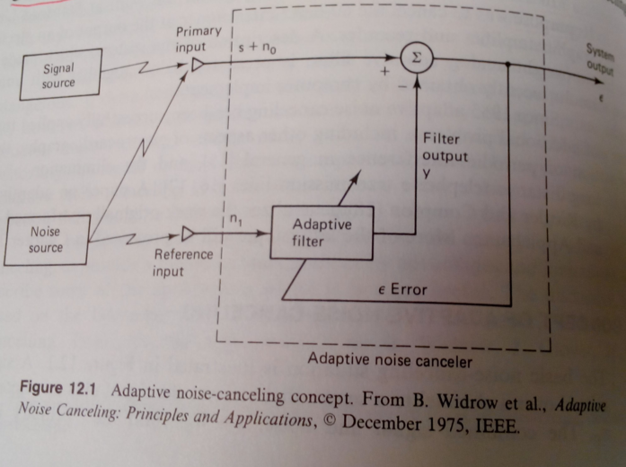
In adapative noise cancelling, we assume the noise source injects into both the primary input and the reference input. THe signal of interest is localized in the primary input. An adaptive filter then tries to reconstruct the noise injected by combining the reference inputs. This approximation (\(y\) in the figure below) is subtracted from the primary input to give the filtered signal (\(\epsilon\)). This filtered output \(\epsilon\) is then fed back into the adaptive filter to tune the filter weights. The rationale is that the perfect adaptive filter will perfectly approximate the noise component \(n_0\), \(\epsilon\) will then become \(s\), and the error signal is minimized.
An interesting question is, why would \(\epsilon\) not be minimized toward 0? If we assume the signal \(s\) is uncorrelated with the noise \(n_0\) and \(n_1\), but \(n_0\) and \(n_1\) are correlated with each other, then the minimum \(\epsilon\) can achieve, in the least mean squared sense, is equal to \(s\). Unfortunately, this results is less intuitive and more easily seen through math (Widrow and Bernard, Ch 12.1).
Another way of seeing LMS filtering is that, in LMS, given an input vector \(\vec{x}\), we multiply it by weights vector \(\vec{w}\) such that we reduce the least-mean-squared error, which is the difference between \(w^T x\) and the desired vector \(\vec{d}\). The error term is then fedback to adjust \(\vec{w}\). This is illustrated below:
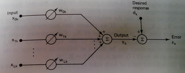
In the case of adaptive filtering, the desired response \(d_k\) is the noise component present in the primary input (\(n_0\)). In fact, for stationary stochastic inputs, the steady-state performance of slowly adapting adaptive filters closely approximates that of fixed Wiener filters.
A side tangent is, why dont we use LMS with Wiener filter in BMI decoding? In this case, the adaptive filter output \(y\) and \(\epsilon\) would have to be decoded covariates, it is difficult to see how that would increase decoding performance.
In contrast with Wiener filter’s derivation where we estimate the gradient of the error in order to find \(\vec{w}\) values to minimize the error, in LMS, we simply aprroximate the gradient with \(\epsilon_k\). This turns out to be an unbiased estimator, and the weights can be updated as:
\[\vec{W_{k+1}} = \vec{W_k} + 2\mu\epsilon_k\vec{X_k}\]where \(\mu\) is the update rate, similar to that in other gradient descent algorithms.
Therefore, the LMS algorithm is a rather simple algorithm to serve as the adaptive filter block in the adaptive noise cancellation framework.
Application in firmware
To apply these algorithms to our headstage application, we treat the current channel’s signal as \(s_n+e_n\), where \(s_n\) is the signal for channel \(n\), \(e_n\) is the noise added to channel \(n\) at current time \(t\). \(e_n\) can be assumed to be Gaussian (even though in reality it probably isn’t, e.g. chewing artifacts). It’s reasonable to assume that \(e_n\) is correlated with noise observed in other channels (since they share the same chip, board, etc): \(e_{n-1}\), \(e_{n-2}\), etc. The signals measured in the previous channels then can be used as the reference input sources to predict and model the current channel’s noise.
This is implemented in the firmware by Tim Hanson as below:
1
2
3
4
5
6
7
8
9
10
11
12
13
14
15
16
17
18
19
20
21
22
23
24
25
26
27
28
29
30
31
32
33
34
35
36
37
38
39
40
41
42
43
44
45
46
47
/* LMS adaptive noise remover
	want to predict the current channel based on samples from the previous 8.
	at this point i1 will point to x(n-1) of the present channel.
		(i2 is not used, we do not need to write taps -- IIR will take care of this.)
	24 32-bit samples are written each time through this loop,
	so to go back 8 channels add m1 = -784
	to move forward one channel add m2 = 112
	for modifying i0, m3 = 8 (move +2 weights)
		and m0 = -28 (move -7 weights)
	i0, as usual, points to the filter taps!
*/
	r3 = abs r3 (v) || r7 = [FP - FP_WEIGHTDECAY]; //set weightdecay to zero to disable LMS.
	r4.l = (a0 = r0.l * r7.l), r4.h = (a1 = r0.h * r7.l) (iss2) || i1 += m1 || [i2++] = r3;
				//saturate the sample, save the gain.

    // apply LMS weights for noise cancelling
	mnop || r1 = [i1++] || [i2++] = r4; //move to x1(n-1), save the saturated sample.
	mnop || r1 = [i1++m2] || r2 = [i0++]; //r1 = sample, r2 = weight.
	a0 = r1.l * r2.l, a1 = r1.h * r2.h || r1 = [i1++m2] || r2 = [i0++];
	a0+= r1.l * r2.l, a1+= r1.h * r2.h || r1 = [i1++m2] || r2 = [i0++];
	a0+= r1.l * r2.l, a1+= r1.h * r2.h || r1 = [i1++m2] || r2 = [i0++];
	a0+= r1.l * r2.l, a1+= r1.h * r2.h || r1 = [i1++m2] || r2 = [i0++];
	a0+= r1.l * r2.l, a1+= r1.h * r2.h || r1 = [i1++m2] || r2 = [i0++];
	a0+= r1.l * r2.l, a1+= r1.h * r2.h || r1 = [i1++m2] || r2 = [i0++];
	r6.l = (a0+= r1.l * r2.l), r6.h = (a1+= r1.h * r2.h) || r1 = [i1++m1] || r2 = [i0++m0];
    // move i1 back to the integrator output 7 chans ago; move i0 back to LMS weight for that chan

	r0 = r0 -|- r6 (s) || [i2++] = r0 || r1 = [i1--] ; //compute error, save original, move i1 back to saturated samples.
	r6 = r0 >>> 15 (v,s) || r1 = [i1++m2] || r2 = [i0++];//r1 = saturated sample, r2 = w0, i0 @ 1
.align 8

    // UPDATE LMS weights
	a0 = r2.l * r7.h, a1 = r2.h * r7.h || nop || nop; //load / decay weight.
r5.l = (a0 += r1.l * r6.l), r5.h = (a1 += r1.h * r6.h) || r1 = [i1++m2] || r2 = [i0--];//r2 = w1, i0 @ 0
	a0 = r2.l * r7.h, a1 = r2.h * r7.h || [i0++m3] = r5; //write 0, i0 @ 2
r5.l = (a0 += r1.l * r6.l), r5.h = (a1 += r1.h * r6.h) || r1 = [i1++m2] || r2 = [i0--];//r2 = w2, i0 @ 1
	a0 = r2.l * r7.h, a1 = r2.h * r7.h || [i0++m3] = r5; //write 1, i0 @ 3
r5.l = (a0 += r1.l * r6.l), r5.h = (a1 += r1.h * r6.h) || r1 = [i1++m2] || r2 = [i0--];//r2 = w3, i0 @ 2
	a0 = r2.l * r7.h, a1 = r2.h * r7.h || [i0++m3] = r5; //write 2, i0 @ 4
r5.l = (a0 += r1.l * r6.l), r5.h = (a1 += r1.h * r6.h) || r1 = [i1++m2] || r2 = [i0--];//r2 = w4, i0 @ 3
	a0 = r2.l * r7.h, a1 = r2.h * r7.h || [i0++m3] = r5; //write 3, i0 @ 5
r5.l = (a0 += r1.l * r6.l), r5.h = (a1 += r1.h * r6.h) || r1 = [i1++m2] || r2 = [i0--];//r2 = w5, i0 @ 4
	a0 = r2.l * r7.h, a1 = r2.h * r7.h || [i0++m3] = r5; //write 4, i0 @ 6
r5.l = (a0 += r1.l * r6.l), r5.h = (a1 += r1.h * r6.h) || r1 = [i1++m2] || r2 = [i0--];//r2 = w6, i0 @ 5
	a0 = r2.l * r7.h, a1 = r2.h * r7.h || [i0++m3] = r5; //write 5, i0 @ 7
r5.l = (a0 += r1.l * r6.l), r5.h = (a1 += r1.h * r6.h) || r1 = [i1++m3] || r2 = [i0--];// inc to x1(n-1) r2 = w1, i0 @ 6
	mnop || [i0++] = r5; //write 6.
This is described by Tim in the following diagram, where \(c\)=current channel number, \(n\)=current sample number.
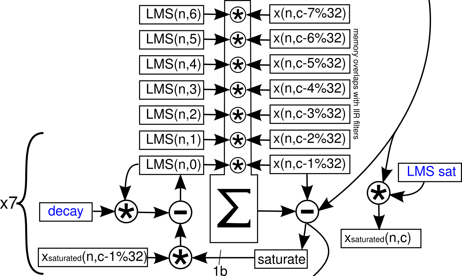
Prior to start of line 12, i1 points to AGC gain of current channel \(c\), i2 points to the integrator mean of current channel, i0 points to AGC transfer function coefficients prior to LMS coefficients.
Line 12: r3 will contain the updated AGC gain, and r7 will contain the weight decay for LMS. The weight decay will be either 0 or 1 in Q15. 0 effectively disables LMS.
Line 13: r0 currently contains AGC output. The multiplication will multiply the AGC output by weight decay, saturate the sample and move it to r4. Updated AGC gain from the previous step is saved by writing to i2, which is then incremented to point at saturated AGC output. i1 is moved to point to the AGC gain value corresponding to channel \((c-7)\%32\).
Line 17: The saturated sample of channel \((n-7)\%32\) is loaded into r1, i1 now points to AGC output for channel \((c-7)\%32\). The current channel’s saturated AGC sample in r4 is saved, and i2 now points to current channel’s AGC-output (from sample n-1).
Line 18: r1 is loaded with AGC output of channel \((c-7)\%32\). i1 points to AGC output of channel \((c-6)\%32\). r2 is loaded with the LMS weight corresponding to channel \((c-7)\%32\), or \(LMS(n,6)\) in diagram.
Line 19: a0 contains the product of \(LMS(n,6)*x(n,c-7\%32)\) in figure above. r1 is loaded with AGC output of channel \((c-6)\%32\) while i1 end up pointing to AGC output of \((c-5)\%32\). r2 is loaded with \(LMS(n,5)\) while i0 end up pointing to \(LMS(n,4)\).
Line 20-24: Continues the adaptive filter operation (the multiply/summation block in diagram). At end of line 24, r1 contains AGC output of \((c-1)\%32\), i1 is moved to point to AGC out of \(c\). r2 is loaded with \(LMS(n,0)\), i0 is moved to point to low-pass filter coefficients.
Line 25: r6 now contains the result of the entire multiply-accumulate operation of the linear combiner (\(y_k\) in figure 2). r1 is loaded with AGC out of current channel, i1 is then moved to point at AGC out of \((c-7)\%32\). r2 is loaded with low-pass filter coefficients and moved back to point to \(LMS(n,6)\). The r1 and r2 values will not be used and will be overwritten next instruction.
Line 28: r0 originally contains current channel’s AGC output. Subtracting r6 from it, r0 will contain the LMS filtered output – \(\epsilon=s+n_0-y\) in figure 1. Meanwhile, the current AGC output is written, after which i2 will point to the delayed sample used for IIR filters. r1 is loaded with AGC out of \((c-7)\), after which i1 points to saturated AGC output of \((c-7)\%32\).
Line 29: After shifting r0 vectorially, r6 is loaded with the sign of filtered LMS output, or \(sign(\epsilon)\). r1 is loaded with saturated AGC output of \((c-7)\%32\), i1 then points to saturated AGC output of \((c-6)\%32\). r2 is loaded with the corresponding LMS weight \(LMS(n,6)\), i0 then points to \(LMS(n,5)\).
Line 33-34: Update the weight \(LMS(n,6)\). r5 will contain the updated weight equal to \(w*\alpha+x*sign(\epsilon)\), where \(w\) is the LMS weight, \(\alpha\) is either 0 or 1 indicating whether LMS is on, \(x\) is the saturated AGC output corresponding to the weight, and \(\epsilon\) corresponds to current channel’s filtered LMS output.
End of line 34, r1 is loaded with saturated AGC output of \((c-6)\%32\), then i1 points to saturated AGC output of \((c-5)\%32\). r2 is loaded with \(LMS(n,5)\), but i0 points to \(LMS(n,6)\).
Line 35: Here the updated \(LMS(n,6)\) weight is written (hence i0 pointing to that location after line 34), after which i0 skips to point at \(LMS(n,4)\).
Line 36: r5 contains the updated weight \(LMS(n,5)\). r1 is loaded with saturated AGC output of \((c-5)\%32\), i1 points to saturated AGC output of \((c-4)\%32\). r2 is loaded with \(LMS(n-4)\), i0 then points to \(LMS(n,5)\) in anticipation of its update.
Line 46: r5 now contains the last updated weight \(LMS(n,0)\). r1 is loaded with current channel’s saturated AGC-output, then i1 is moved to point current channel’s delayed sample (in anticipation of IIR filter). i0 points to \(LMS(n,0)\).
Line 47: The updated \(LMS(n,0)\) is written back to memory.
The implemented algorithm is a modified LMS approach, where the filter weights are updated by \(\begin{align} \vec{W_{k+1}} &= \vec{W_k} + \vec{X_k}*sign(\epsilon_k) \\ &= r2*r7 + r1*r6 \end{align}\)
where the registers are those used in line 33-46.
Here, the old \(w_k\) are loaded into r2. r7 contains a weight-decay factor. If it’s set to 0, LMS is effectively disabled as no weight update would happen and it becomes a fixed gain stage.
r1 contains the saturated version of each reference channel’s input. r6 is the sign of the error term.
In this modified LMS approach, if both the error and sample are the same sign, the weight would increase (Hebb’s rule). This implementation involves saturation and 1-bit weight updates, so it’s not analytical. However, it is fast and according to Tim,
in practice the filter settles to final weight values within 4s. The filter offers 40dB of noise rejection.
If at any time the error term \(\epsilon_k=0\), that means the current channel can be completely predicted by the previous 7 channels, that means the current channel is measuring only noise. This could serve as a good debugging tool.
Finally, at the end of this code block, r0 contains the LMS filtered sample, also \(\epsilon\). The IIR stage following LMS then operates directly on this filtered sample. Therefore only the regular and saturated AGC outputs are saved, while the LMS filter output is not saved until the IIR stage as a delayed sample (after AGC-out slot).
Effects of removing LMS
LMS is now implemented with RHD headstages in radio_AGC_LMS_IIR_SAA.asm.
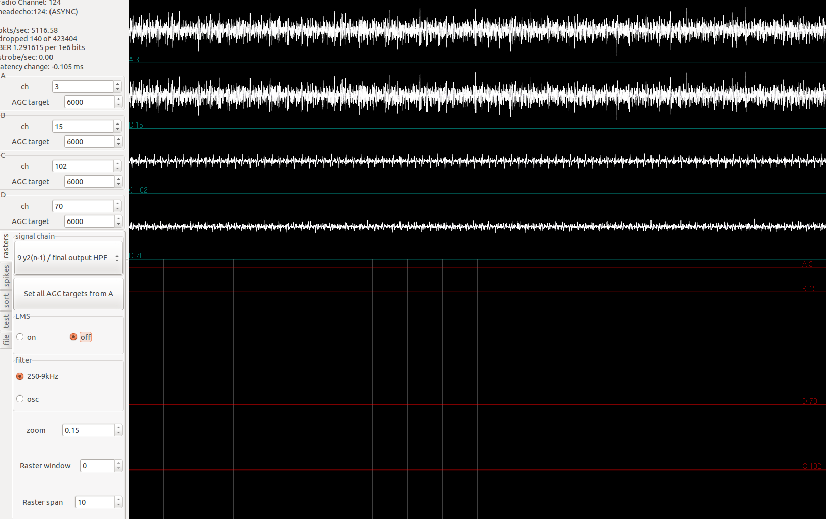
The effects of LMS is especially clear when all the channels of an amplifier is applied the same signal:
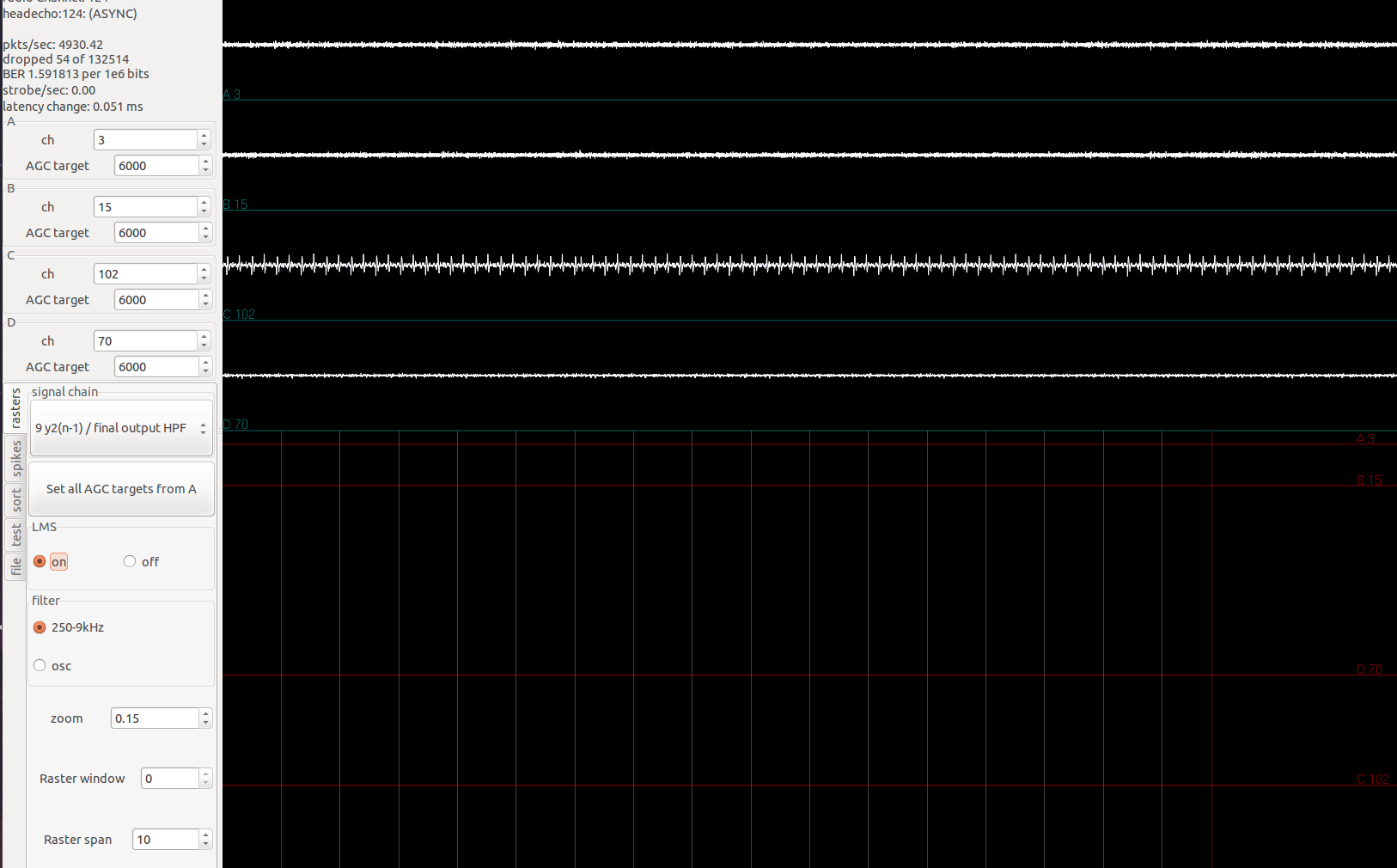
Simulated spike signals are being applied through the Plexon headstage tester to channel 0-31. In image shown, the first two channels have fairly low signal. This is expected since all channels have the same signal, the previous 7 channels can exactly reconstruct the signal in the current channel, subtraction leaves little left.
Turning off LMS, we have the following:
The identical spike signals applied now show up loud and clear in the first two channels shown.