
While recent work such as A wireless transmission neural interface system for unconstrained non-human primates focuses on the how transmitted analog waveform compares to that recorded by wired commerical systems, our validation goal is somewhat different.
While our wireless system operates also streams full analog waveforms, the focus is on onboard spike sorting and reporting spikes. Therefore, the most important measure is how the reported spike trains compares with that of the ground truth and that sorted/measured by commercial wired systems. Thus spike-train analysis is conducted here.
Systems compared:
- RHA-headstage with resistor-set RHA-Intan filtering, AGC, and four stages of IIR digital filtering. Final bandwidth is 500Hz-6.7kHz or 150Hz-10kHz.
-
RHD-headstage with onchip-resistor-set RHD-Intan filtering (1Hz-10kHz), manually set fixed gain (Q7.8 ranges -128:0.5:127.5), and two stages of IIR digital filtering. Final bandwidth is 250Hz-9kHz.
I observed it’s much easier to do spike sorting keeping the Intan onboard bandpass filter to have wide bandwidth, so the displayed waveform is not too distorted. The IIR filters can apply sufficient filtering to remove low and high frequency noise to expose the key spike features. But having access to the signal prior to IIR can be very helpful for sorting, especially when SNR is low. Finally, changing from AGC to user-set fixed gain seems to yield much cleaner signals since AGC amplifies noise as well, making it very difficult to sort under low SNR. Downside is it’s neccessary to check the templates often to make sure the previously set gain is enough.
- Plexon (old Harveybox..), standard spike filtering options. Waveform uses 20kHz sampling rate.
All three systems use manual PCA spike sorting. While the actual sorting interface has a time window of 1ms, the headstages use only templates that are 0.5ms long to sort spikes onboard.
Measures used:
To compare spike train performance, I referred to A comparison of binless spike train measures; Paiva, Park, Principe 2010 for a review and comparison of these measures. Very useful despite an amateur error with one of the formulas.
-
The first binless distance measure proposed in the literature. Defines the distance between two spike trains in terms of the minimum cost of transforming one spike train into the other by means of just three basic operations: spike insertion (cost 1), spike deletion (cost 1), and shifting a spike by some interval by \(\Delta t\)(cost \(q\|\Delta t\|\)). The cost per time unit, \(q\) sets the time scale of the analysis. For \(q=0\) the distance is equal to the difference in spike counts, while for large \(q\) the distance is linearly proportional with the number of non-coincident spikes, as it becomes more favorable to delete and reinsert all non-coincident spikes rather than shifting them (cost 2 in this instance). Thus, by increasing the cost, the distance is transformed from a rate distance to a temporal distance. Note that the cost is inversely proportional to the acceptable time shift between two spikes.
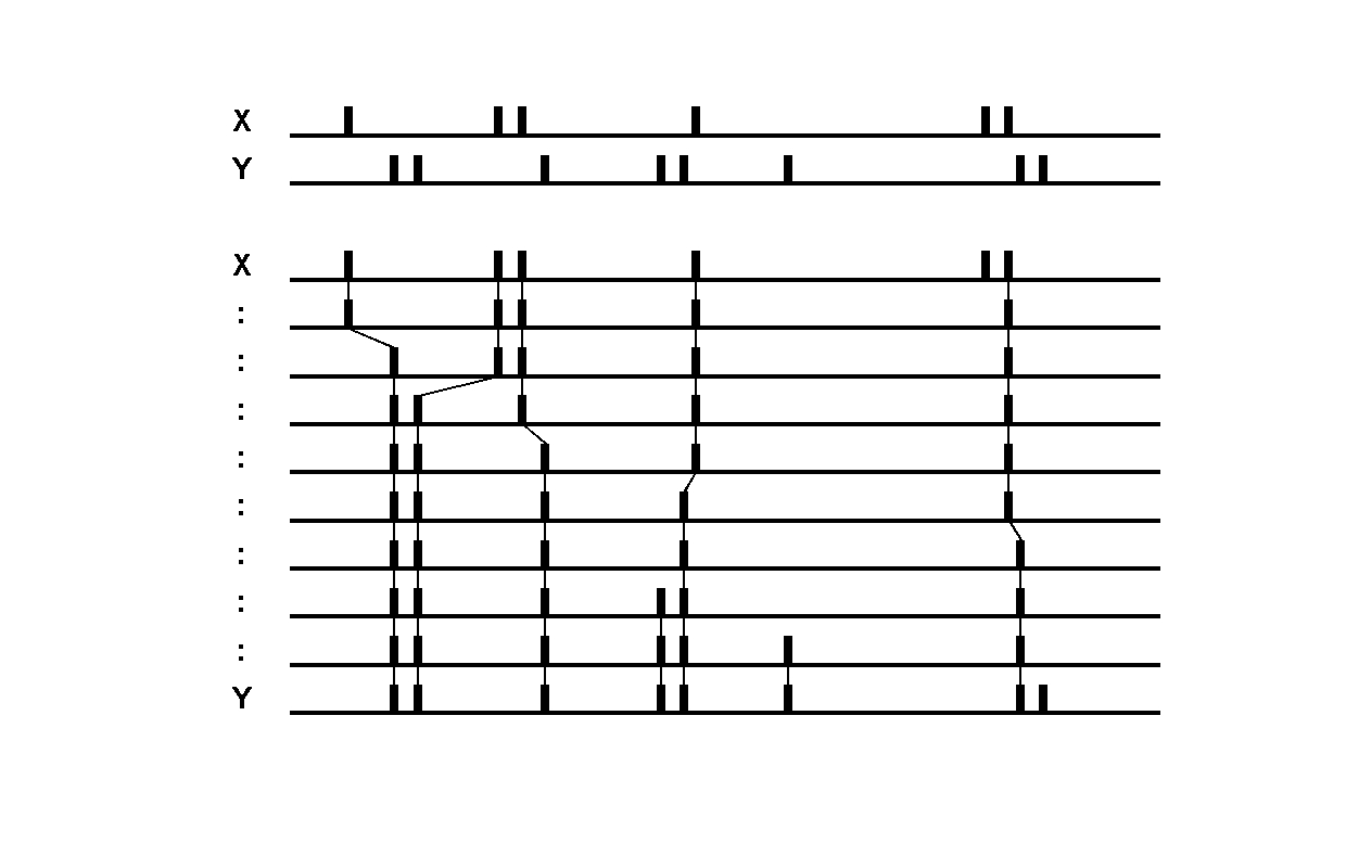 Victor-Purpura spike train distance. Two spike trains X and Y and a path of basic operations (spike deletion, spike insertion, and spike shift) transforming one into the other. (Victor and Purpura, 1996).
 -
Similar to the VP-distance, VR distance utilizes the full resolution of the spike times. The VR distance is the Euclidean distance between exponentially filtered spike trains.
A spike train \(S_i\) is defined as \(S_i(t)=\sum_{m=1}^{N_i} \delta(t-t_m^i)\), where \(\{t_m^i:m=1,...,N_i\}\) are the spike times.
After convolving this spike train with a causal decaying exponential function \(h(t)=exp(-t/\tau)u(t)\), we get the filtered spike train \(f_i(t)=\sum_{m=1}^{N_i} h(t-t_m^i)\). The Van Rossum distance between two spike trains \(S_i\) and \(S_j\) is the Euclidean distance:
\[d_{vR}(S_i,S_j)=\frac{1}{\tau}\int_0^{\infty} [f_i(t)-f_j(t)]^2 dt\]For VR, the parameter \(\tau\) sets the time scale, which can be though of as inversely related to VP’s \(q\) parameter. The metric acts as a count of non-coincident spikes (temporal relationship) to a difference in spike count (spike rates) as the kernel size \(\tau\) is increased. This is opposite of what happens to VP distance as \(q\) is increased.
-
Schreiber-correlation dissimilarity
The Schreiber dissimilarity based on the correlation measure defined in terms of Gaussian-filterd spike trains. In this approach, the filtered spike train \(S_i\) becomes \(g_i(t)=\sum_{m=1}^{Ni} G_{\sigma/\sqrt{2}}(t-t_m^i)\), where \(G_{\sigma/\sqrt{2}}(t)=exp(-t^2/\sigma^2)\) is the Gaussian kernel. The role of \(\sigma\) here is similar to \(\tau\) in Van Rossum distance, and is inversely related to \(q\) in VP distance. Assuming a discrete-time implementation of the measure, then the filtered spike trains can be seen as vectors, for which the usual dot product can be used. Therefore a correlation like dissimilarity measure can be derived:
\[d_{CS}=1-r(S_i,S_j)=1-\frac{\vec{g_i}\cdot\vec{g_j}}{\|\vec{g_i}\|\|\vec{g_j}\|}\]This metric is always betweeen 0 and 1, and can be thought of as a measure of the angle between the two filtered spike trains. Note that this quantity is not a strict distance metric because it does not fulfill the triangel inequality. Chicharro 2011 suggests that this measure’s applicability to estimate reliability is limited because of the individual normalization of spike trains, which renders the measure sensitive only to similarities in the temporal modulation of the individaul rate profiles but neglects differences in the absolute spike count.
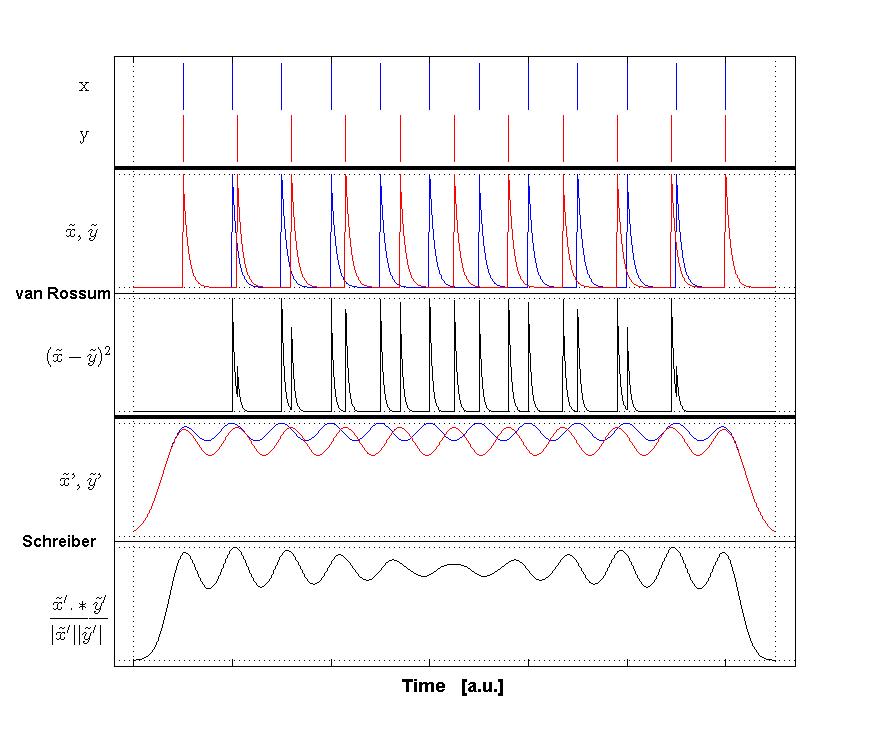 Van Rossum spike train distance and Schreiber et al. similarity measure. Figure from (van Rossum, 2001) and (Schreiber et al., 2003)
 -
Binned distance (\(d_B\))
While both Paiva2010 and Chicharro2011 recommends not using a binned method to measure spike train similarity, it is more directly related to BMI methods. The binned distance is simply the sum of the absolute value of the two binned spike trains, which would require us to compare spike trains of the same length.
Notes
According to simulation tests conducted by Paiva 2009, none of the above measures performs the best or consistently when measuring different aspects of spike-train similarity, including 1) discriminating different firing rate; 2) discriminating changing firing rate; 3) Spike train synchrony. In the end, Paiva concludes:
- VP and van Rossume distances perform better discriminating constant firing rate.
- Schreiber and binned-distance perform better discriminating synchrony.
- All measures performed similar in discriminating instantaneous firing rates.
Ideally, validation should tell us exactly what percentage of detected spikes are true positives, and how many spikes we have missed. But that requires probabilistic calculation (e.g. is a spike false positive, or just a shifted spike) that is difficult, I settle for these metrics that are well established and are relevant for BMI – the firing rates are usually binned and normalized prior to decoding, which is sensitive to time scales. There are other time-scale independent spiket rain distances such as event synchronization (Quiroga 2002), SPIKE synchronization (Kreuz 2015), ISI-distance (Kreuz 2007a), and SPIKE-distance (Kreuz 2013), but they are in my opinion harder to interpret.