I can apply linear algebra, but often forget/confuse the spatial representations.

A good resource is Gilbert Strang’s essay. I remember him talking about this when I took 18.06, but he was old at that point, and I barely went to class. So I didn’t retain much. This notes of his still retains his stream of consciousness style, but the two diagrams summarizes it well, and is useful to often go back and make sure I still understand it.

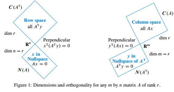
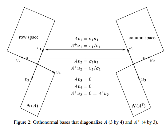
The first one shows the relationship between the four subspaces of a matrix \(A\). The second one adds in the relationship between the orthonormal basis of the subspaces.

Strang concludes:

Finally, the eigenvectors of \(A\) lie in its column space and nullspace, not a natural pair. The dimensions of the spaces add to \(n\), but the spaces are not orthogonal and they could even coincide. The better picture is the orthogonal one that leads to the SVD.

The first assertion is illuminating. Eigenvectors \(v\) are defined such that \(Av=\lambda v\). Suppose \(A\) is \(M\times N\), then \(v\) must be \(M\times 1\), therefore eigenvectors only work when \(M=N\). On the other hand, in SVD, we have \(A=U\Sigma V^T\) and

• \(Av_i=\sigma_i u_i\) for \(i=1,...,r\), where \(r\) is the rank of column and row space.

  \(u_i\) are the basis for the column space (left singular vectors), \(v_i\) are the basis for the row space (right singular vectors).

  The dimensions for this equation matches because the column space and row space are more natural pair.

• \(Av_i=0\), \(A^Tu_i=0\), for \(i>r\).

  \(v_i\) are the eigenvectors of the null space of \(A^T\),

  \(u_i\) are the eigenvectors of the null space of \(A\).

  They also match up similarly (Figure 2).

• In \(Ax=b\), \(x\) is in the row space, \(b\) is in the column space.
• If \(Ax=0\), then \(x\) is in the null space (kernel) of A, and is orthogonal complement of the row space of A, \(C(A^T)\).
• In \(A^Tx=b\), \(x\) is in the column space, \(b\) is in the row space.
• If \(A^Tx=0\), then \(x\) is in the cokernel of A, and is orthogonal complement of the column space of A, \(C(A)\).

Relationship with PCA ***

PCA Algorithm Inputs: The centered data matrix \(X\) and \(k\gt1\).

1. Compute the SVD of \(X\): \([U,\Gamma,V]=svd(X)\).
2. Let \(V_k=[\mathbf{v}_1,...,\mathbf{v}_k]\) be the first \(k\) columns of \(V\).
3. The PCA-feature matrix and the reconstructed data are: \(Z=XV_k, \hat{X}=XV_kV_k^T\).

So in PCA, the rows of the data matrix are the observations, and the columns are in the original coordinate system. The principle components are then the eigenvectors of the row space. We can do PCA in MATLAB with pca or manually with svd:

1
2
3
4
5
6
7
8
9
10
11
12
13
14
15
16
17
18
19
20
21
% PCA test
a = rand(100,1);
b = 5*a+rand(100,1);

data = [a, b];  % rows are observations
plot(a,b, '.');


% PCA results
% coeffs=PC in original coordinate[PxP], 
% scores=observation in PC-space [NxP], 
% latent=variance explained [Px1]
[coeffs, score, latent] = pca(data);
hold on;
plot(score(:,1), score(:,2), 'r.');

% SVD results
centeredData = bsxfun(@minus, data, mean(data,1));
[U, S, V] = svd(centeredData);
svd_score = centeredData*V;
plot(svd_score(:,1), svd_score(:,2), 'g.');

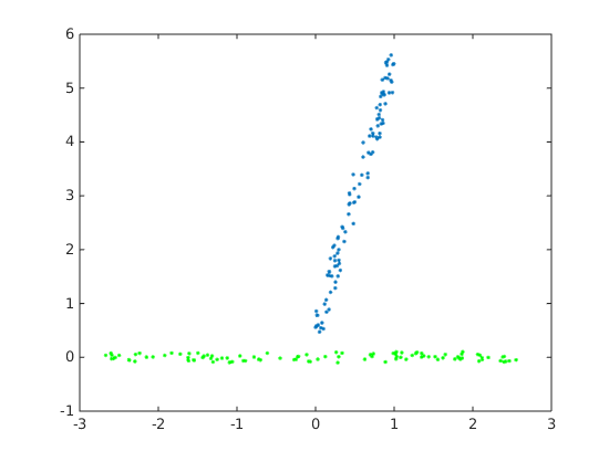
The results shown below. Blue is original data, green/red are the PCA results, they overlap exactly. Note that MATLAB’s pca by default centers the data.

Projection into subspace (e.g. Kaufman 2014, Cortical activity in the null space, Even-Chen 2017, Neurally-driven error detectors) ***

Suppose we have a trial-averaged neural activity matrix \(A\) of size \(N\times T\), where \(N\) is number of neurons, and \(T\) is number of time bins.

In online BMI experiment, a linear decoder maps the neural activity vector \(n_t\) of size \(N\times 1\) to kinematics \(v_t\) of size \(2\times 1\) via the equation \(v_t = w n_t\), where \(w\) is of size \(2\times N\).

Kaufman describes the output-potent neural activities as collection of \(n_t\) such that \(v_t\) is not null. Therefore the output-potent subspace of \(n_t\) is the rowspace of \(w\). Similarly, the output-null subspace is the null space of \(w\).

By projecting the activity matrix \(A\) into these subspaces, we can get an idea of how much variance in the neural activities can be accounted for the modulation to control actuator kinematics:

1. Use SVD on \(w=U\Sigma V^T\) to get its row and null space, defined by the first \(r\) columns of \(V\) (call it \(w_{potent}\)), and the last \(N-r\) columsn of \(V\) (call it \(w_{null}\)), respectively, where \(r\) is the rank of \(w\).
2. Left multiply \(A\) by these subspaces (defined by the those columns) to get \(A_{potent}\) and \(A_{null}\).
3. The variance of \(A\) explained by projection into the subspaces is obtained by first subtracting each row’s mean from each matrix, then taking the L2 norm of the entire matrix (Frobenius norm of the matrix).

Philip Sabes’ Linear Algebra notes