Reading List

Wiener Filter

Wiener filter is used to produce an estimate of a target random process by LTI filtering of an observed noisy process, assuming known stationary siganl and noise spectra. This is done by minimizing the mean square error (MSE) between the estimated random process and the desired process.

Wiener filter is one of the first decoding algorithms used with success in BMI, used by Wessberg in 2000.

Derivations of Wiener filter are all over the place.

Many papers and classes refer to Haykin's Adaptive Filter Theory, a terrible book, in terms of setting the motivation, presenting intuition, and the horrible typesetting.
MIT's 6.011 notes on Wiener Filter has a good treatment of DT noncausal Wiener filter derivation, and includes some practical examples. Its treatment on Causual Wiener Filter, which is probably the most important regarding real-time processing, is mathematical and really obscures the intuition -- we reach this equation from completing the square and using Parseval's theorem, without mentioning the consquences in the time domain. My notes
Max Kamenetsky's EE264 notes gives the best derivation and numerical examples of the subject for practical application, even though only DT is considered. It might get taken down, so extra copy [here](/reading_list/assets/wienerFilter.pdf}. Introducing the causual form of Wiener filter using input whitening method developed by Shannon and Bode fits into the general framework of Wiener filter nicely.

Wiener Filter Derivation Summary

Both the input $x$ (observation of the target process) and output $y$ (estimate of the target process $d$ , after filtering) are random processes.
Derive expression for cross-correlation between input and output.
Derive expression for the MSE between the output and the target process.
Minimize expression and obtain the transfer function in terms of $S_{xx}$ and $S_{xd}$ , where $S$ are Z or Laplace transforms of the cross-correlations.

This looks strangely similar to a linear regression. Not surprisingly, it is known to statisticians as the multivariate linear regression.

Kalman Filter

In Wiener Filter, it is assumed that both the input and target processes are WSS. If not, one may assume local stationarity and conduct the filtering. However, nearly two decades after Wiener's work, Rudolf Kalman developed the Kalman filter, which is the optimu mean square linear filter for nonstationary processes (evolving under a certain state space model) AND stationary ones (converging in steady state to Wiener filter).

Two good sources on Kalman Filter:

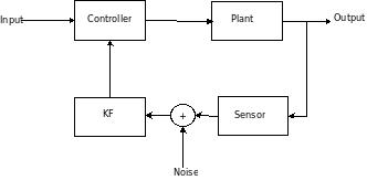
Dan Simon's article describes the intuition and practical implementation of KF, specifically in an embedded control context. The KF should be coupled with a controller when the sensor reading is unreliable -- it filters out the sensor noise. My notes
Greg Welch and Gary Bishop's An Introduction to the Kalman Filter. Presents just the right amount of math in the derivation of the KF. My notes
Update (12/9/2021): New best Kalman Filter derivation, by Thacker and Lacey. Full memo, Different link.

The general framework of the Kalman filter is (using notation from Welch and Bishop):

\begin{aligned} x_{k} & = A x_{k - 1} + B u_{k - 1} + w_{k - 1} \\ z_{k} & = H x_{k} + v_{k} \\ p (w) & \approx N (0, Q) \\ p (v) & \approx N (0, R) \end{aligned}

The first equation is the state model. $x_{k}$ denotes the state of a system, this could be the velocity or position of a vehicle, or the desired velocity or position of a cursor in BMI experiment. $A$ is the transition matrix -- describes how the state will transition depending on past states. $u_{k}$ is the input to the system. $B$ describes how the inputs are coupled into the state. $w_{k}$ is the process noise.

The second equation is the observation model - it describes what kind of measurements we can observe from a system with some state. $z_{k}$ is the measurement, it could be the speedometer reading of the car (velocity would be the state in this case), or it could be neural firing rates in BMI (kinematics would be the state). $H$ is the observation matrix (tuning model in BMI applications). $v_{k}$ is the measurement or sensor noise.

One caveat is that both $w$ and $v$ are assumed to be Gaussian with zero mean.

The central insight with Kalman filter is that, depending on whether the process noise or sensor noise dominates, we weigh the state model and observation model differently in their contributions to compute the new underlying state, resulting in a posteriori state estimate \[\hat{x_k}=\hat{x_k}^- + K_k(z_k-H\hat{x}_k^-)\] Note the subscript $_{k}$ denotes at each discrete time step.

The first term ${\hat{x_{k}}}^{-}$ is the contribution from the state model - it is the a priori state estimate based on the state model only. The second term is the contribution from the observation model - given the a posteriori state estimate.

Note a priori denotes a state estimate at a given time state $k$ to use only knowledge of the process prior to step $k$ . a posteriori denotes a state estimate that also uses the measurement at step $k$ , $z_{k}$ .

K$$ is the Kalman gain, the derivation of which is the most mathematically involved step. The derivation involves the definition of:  1. $P_K^-$: the *a priori* estimate error covariance \\[P_k^-=E[e_k^-e_k^{-T}]=E[(x_k-\hat{x_k}^-)(x_k-\hat{x_k}^-)]\\].  2. $P_K$: the *a posteriori* estimate error covariance \\[P_k=E[e_ke_k^T]=E[(x_k-\hat{x_k})(x_k-\hat{x_k})^T]\\].   To derive $K$, we want to minimze the *a posteriori* state estimate $P_K$, which makes intuitive sense. A good estimate of the state is one that minimizes the variance of the estimation error. A bunch of math later, we obtain \\[K_k=P_k^-H^T(HP_k^-H^T+R)^{-1}\\].  Looking at the *a posteriori* state estimate equation, we can see that   1. If the sensor noise is extremely low, i.e. $R\rightarrow 0$, then we should trust the sensor reading, and $\hat{x_k}$ should just be $H^{-1}z_k$. This is indeed the case as $\lim_{R_k\to 0}K_k=H^{-1}$.  2. If the process noise is extremely low, i.e. $Q\rightarrow 0$, then we should trust the state model on how the state should change, thus $\hat{x_k}$ should just equal to the *a priori* state estimate $\hat{x_k}^-$. This is indeed the case as $\lim_{P_k^-\to0}K_k=0$.  In implementation, KF operates by alternating between the prediction phase and a correct phase. The prediction phase projects the state based on the state model. The correction phase updates the estimate from the predictioin phase by the measurement and observation model. Operation is recursive and efficient.  ![KF_architecture](/reading_list/assets/KF_diagram.jpg){: .center-image }  Thus the KF is a generalization of the Wiener filter when the input and reference processes are non-stationary. This is done by estimating the *state*, tracking the changing statistics in the non-stationary process. This tracking is enabled by the incorporating the measurements taken.  KF is superior to Wiener Filter also because   1. There are less parameters to be fitted. 2. The movement and observation models are decoupled, providing more flexibility in system design.  **Extended Kalman Filter (EKF)**  The default KF addresses the general problem of trying to estimate the state $x$ goverend by a *linear* stochastic model. However, when the state and/or observation model is nonlinear, the KF needs to linearize about the current mean and covariance.  Therefore, $A$, $B$, $H$, $w$ and $v$ need to be replaced by the Jacobians linearized at the current mean and covariance. The math is different, but the architecture is the same.  **Unscented Kalman Filter (UKF)**  UKF is used a better implementation of KF for nonlinear state and observation model. Why use UKF when we can use EKF?  According to [wikipedia](https://en.wikipedia.org/wiki/Kalman_filter#Unscented_Kalman_filter), whe the state and observation models   > are highly non-linear, the extended Kalman filter can give particularly poor performance. This is because the covariance is propagated through linearization of the underlying non-linear model. The unscented Kalman filter (UKF) uses a deterministic sampling technique known as the unscented transform to pick a minimal set of sample points (called sigma points) around the mean. These sigma points are then propagated through the non-linear functions, from which the mean and covariance of the estimate are then recovered. The result is a filter which more accurately captures the true mean and covariance.   In Zheng Li's 2009 paper, [Unscented Kalman Filter for Brain-Machine Interfaces](http://journals.plos.org/plosone/article?id=10.1371/journal.pone.0006243), he applies the UKF to BMI. The keypoints were:  1. UKF allows nonlinear neuron tuning model -- this is a nonlinear observation model. In the paper, the tuning model is quadratic and describes the tuning better than a linear one.  2. UKF also allow a nonlinear movement model -- nonlinear state model.  3. The movement model was made to be of *degree-n*, meaning that the state equation is no longer a function of the previous state, but of the previous *n* states. Incorporating this "movement history" acts as smoothing for the output kinematics.  The number of sigma points was chosen to be $2d+1$, where $d=4n$ is the dimension of the state space. If $n=10$, then $d=40$, big state space.  The name *unscented* is pretty dumb and provides no clue to how it modifies the KF.  **Adaptive UKF**  As a follow up to the 2009 paper, Li published [Adaptive UKF](http://www.ncbi.nlm.nih.gov/pmc/articles/PMC3335277/). This algorithm modifies on the n-degree UKF by including   > Bayesian regression self-training method for updating the parameters of an unscented Kalman filter decoder. This novel paradigm uses the decoder’s output to periodically update the decoder’s neuronal tuning model in a Bayesian linear regression.   So, the tuning model/observation matrix $H$ is updated online periodically. Great for modeling the plasticity associated non-stationarity.  **ReFIT-KF**