Wireless Project github

While trying to confirm that the radio transmission for the RHD-headstage firmware was working correctly, I needed a way to decouple the signal-chain from the transmission in terms of testing. A nice side-effect of the cascading biquad IIR filter implementation is that, by writing coefficients for the biquads in a certain way, sinusoidal oscillations for different frequencies can be generated. If this was done on the last biquad, it would result in pure sinusoids being transmitted to gtkclient (when the final output is selected for transmission, of course), and it would be easy to see if the data is getting corrupted in the transmission process (if not, then any corruption would be due to the signal-chain code).

Below is the the DI-biquad block diagram again:

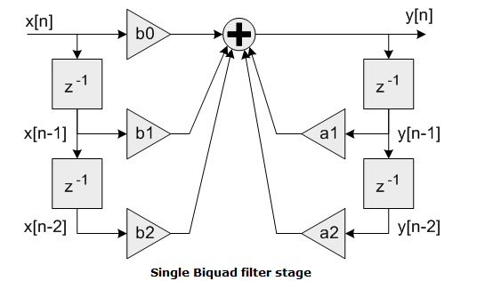
If we assume nonzero initial conditions such that \(y[n-1]\) and \(y[n-2]\) are nonzero, then pure oscillations can be induced by setting \(b_0\), \(b_1\) and \(b_2\) to be 0, in which case only feedback is present in the biquad.

The system function is then:

Let \(a_1=2-f_p\), and \(a_2=-1\), then the resulting conjugate poles will be at

The resulting normalized frequency of oscillation is \(\omega=\angle{p_1}\), in radians/sample. Oscillation frequency in Hz is \(f=\frac{\omega F_s}{2\pi}\), where \(F_s\) is the sampling frequency (in our case 31.25kHz for all channels).

So all we need to find is \(fp\) to get a desired oscillation frequency. To find the appropriate coefficients for the last biquad of my signal to induce oscillations, I used the following Matlab script. Note that the coefficients naming is different from that in the diagram – \(a_0\) and \(a_1\) in script are the same as \(a_1\) and \(a_2\) in diagram.

1
2
3
4
5
6
7
8
9
10
11
12
13
14
15
16
17
18
19
20
21
22
23
24
25
26
27
28
 
% IIR oscillator - myopen_multi/gktclient_multi/matlab/IIR_oscillator.m
Fs = 31250;     % sampling frequency

% To get oscillator of frequency f, do:
% set b0=0, b1=0, a1=-1, and a0=2-fp
fp = 0.035;
omega = angle((2-fp+sqrt(fp^2-4*fp))/2); % in rad/sample
f = omega * Fs/(2*pi);  % convert to Hz

% But a0 is fixed-point number, convert fp:
fp_fixed = round(fp*2^14);

% coefficients
b0 = 0;
b1 = 0;
a0 = (2^15-fp_fixed)/2^14;
a1 = -1;

y = [0.5, 0.5];       % y[n-1]=0.5, y[n-2]=0.5
x = rand(1,1002)*2;   % 1000 random values, including x[n-1] and x[n-2]

for i=3:numel(x),
    val = b0*x(i) + b1*x(i-1) + b0*x(i-2) + a0*y(i-1) + a1*y(i-2);
    y = [y, val];
end

plot_fft(y, 31250);

In line 10, \(f_p\) is converted to a number that can be represented by Q14 (see biquad IIR filter implementation for why).

Line 19-27 simulates running a biquad with the newly found coefficients, and plots the FFT of the output waveform.