Linear model is a crazy big subject, dividing into:

• LM (linear models) – this includes regressions by ordinary least squares (OLS), as well as all analysis of variance methods (ANOVA, ANCOVA, MANOVA). Assumes normal distribution of the dependent variable.

• GLM (generalized linear models) – linear predictor and dependent variable related via link functions (poisson, logistic regressions fall into this category).

ANOVA and friends (and their GLM analogs) in GLM and LM are achieved through the introduction of indicator variables representing “factor levels”.

• GLMM (generalized linear mixed models) – Extension of GLMs to allow response variables from different distributions. Mixed refers to both fixed and random effects.

A book that seems to have reasonable treatments on the connections is ANOVA and ANCOVA: A GLM approach.

MANOVA, repeated measures, and GLMM

Repeated measures is when the same set of subjects, divided into different treatment groups, are measured over time. It would be silly to treat all of the measurements as independent. Advantage is there is less variance bebetween measurements taken on the same subject. Consequently, a repeated measures design allow for same statistical power with less subjects (compared to another design where N different subjects are measured at the different time points and treating all these measurements as independent).

This can be achieved through:

1. MANOVA approach - The measurements of all subjects at a given time is a length-n vector and becomes the dependent variable of our MANOVA.

2. GLMM - controls for non-independence among the repeated observations for each individual by adding one or more random effects for individuals to the model.

Good explanation

Variance, Deviance, Sum of Squares (SS), Clustering, and PCA

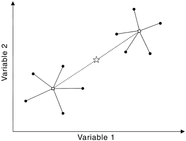
In LM and ANOVA-based methods, we try to divide the total sum of squares (measuring the response deviation of all data points from the grand mean) into components that can be explained by the predictor variables. A good mental picture to have is:

.

Don’t mind that it is in 2D, it actually illustrates the generalization of ANOVA into MANOVA. In ANOVA, response values are distributed along a line, in MANOVA, response values are distributed in n-dimensional space. As we see here, the within-group sum of squares (SSW) is the sum of squared distances from individual points to their group centroid. The among-group sum of squares (SSA) is the sum of squared distances from group centroids to the overall centroid. In ANOVA methods, a predictor’s effect is significant if the F-test statistic, proportional to the ratio of SSA and SSW hits the critical value.

The analogous method is the analysis of deviance in GLM methods, where we are comparing likelihood ratios instead of SS ratios. Still a bitch though.

This framework of comparing dissimilarity or distance is very useful, especially in constructing randomization-based permutation tests. The excellent paper by Anderson 2001 describes how to use this framework to derive a permutation-based non-parametric MANOVA test. This was implemented in MATLAB in the Fathom toolbox.

A key insight is as shown in the following picture

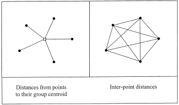
The sum of squared distances from individual points to their centroid is equal to the sum of squared distances divided by the number of points. Why is this important? Anderson explains:

In the case of an analysis based on Euclidean distances, the average for each variable across the observations within a group constitutes the measure of central location for the group in Euclidean space, called a centroid. For many distance measures, however, the calculation of a central location may be problematic. For example, in the case of the semimetric Bray–Curtis measure, a simple average across replicates does not correspond to the ‘central location’ in multivariate Bray–Curtis space. An appropriate measure of central location on the basis of Bray–Curtis distances cannot be calculated easily directly from the data. This is why additive partitioning (in terms of ‘average’ differences among groups) has not been previously achieved using Bray–Curtis (or other semimetric) distances. However, the relationship shown in Fig. 2 can be applied to achieve the partitioning directly from interpoint distances.

Brilliant! Now we can use any metric – SS, Deviance, absolute value, to run all sorts of tests. Note now we see how linear models are similar to clustering methods, but supervised (i.e. we define the number of clusters by the number of predictors).

PCA

PCA is pretty magical. Bishop’s Pattern Recognition and Machine Learning devotes an entire chapter (12) on it, covering PCA as:

1. Projecting data to subspace to maximize the projected data’s variance. This is the traditional and easiest approach to understand.

2. A complementary formulation to the previous one is projecting data to subspace to mimimize the projection error. This is basically linear regression by OLS. There is even a stackexchange question on it.

3. Probabilistic PCA. In this approach, PCA is described as the maximum likelihood solution of a probabilistic latent variable model. In this generative view, the data is described as samples drawn according to

   \[p(\mathbf{x}|\mathbf{z})=\mathscr{N}(\mathbf{x}|\mathbf{W}\mathbf{z}+\mathbf{\mu}, \sigma^2\mathbf{I})\]

   This is a pretty mind blowing formulation which would link PCA, traditionally a dimensionality reduction technique, with factor analysis that describe latent variables. There is a big discussion on stackexchange on this generative view of PCA.

4. Bayesian PCA. Bishop is a huge Bayesian lover, so of course he talks about making PCA Bayesian. A cool advantages is automatic selection of principal components by giving the vectors of \(W\) a prior which is then shrunk during the EM procedures. Another cool thing about PPCA/Bayesian PCA is the iterative procedure allows estimating the top principal components without computing the entire covariance matrix/eigenvalue decomposition.

5. Factor Analysis. This is treated as a generalization of PPCA, where instead of \(\sigma^2\mathbf{I}\), we have

   \[p(\mathbf{x}|\mathbf{z})=\mathscr{N}(\mathbf{x}|\mathbf{W}\mathbf{z}+\mathbf{\mu}, \mathbf{\Psi})\]

   where \({\Psi}\) is still a diagonal matrix, but the individual variance values are not the same. This has the following consequences of using PCA vs. FA, quoting amoeba,

   As the dimensionality n increase, the diagonal [of sampling covariance matrix] becomes in a way less and less important because there are only n elements on the diagonal and O(n^2) elements off the diagonal. As a result, for the large n there is usually not much of a difference between PCA and FA at all […] For small n they can indeed differ a lot.

Nonparametric tests and Randomization tests

Here is a nice chart from Kording lab’s page.

One common misconception among neuroscientists (and me, until a short while ago) is to use conventional non-parametric tests such as WIlcoxon, Mann-Whitney, Kruskal-Wallis, etc as a cure-all for violation of assumptions in the parametric tests. However, these tests simply replace the actual response values by their ranks, then proceed with calculating sum of squares, and using a \(Chi^2\) test statistic instead of an F-test.

However, as Petraitis & Dunham 2001 points out,

The Chi-squared distribution of the test statistic is based on the assumption that ranked data for each treatment level are samples drawn from distributions that differe only in location (e.g. mean or median). The underlying distributions are assumed to have the same shape (i.e. all other moments of the distributions– the variance, skewness, and so on – are identical). These assumptions about nonparamteric tests are often not appreciated, and ecologists often assume that such tests are distribution-free).

Hence the motivation for many permutation based tests, which Anderson notes can detect both variance and location differences (but not correlation difference). Traditional parametric tests, on the other hand, are also sensitive to correlation and dispersion differences (hence why everyone loves them).