
I have the data shown below 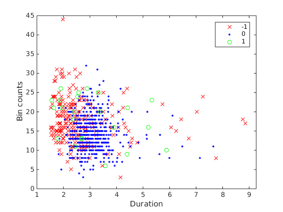 , where the dependent variable is the count data Bin counts (
bincnts), and vary with categorical predictor duration, and covariate reward_cond (shown by the colors). Traditionally, this would call for 1-way Analysis of Covriance (ANCOVA), which is essentially ANOVA but with a covariate. Intuitively, ANCOVA fits different regression lines to different groups of data, and check to see if the categorical variable has a significant effect on the intercept of the fitted regression lines (insert some pictures)
ANCOVA has the model assumptions that:
- Homogeniety of slopes.
- Normal distribution of the response variable.
- Equal variance due to different groups.
- Independence
My data clearly violates (2), being count data and all.
I could do a permutation based ANCOVA, as outlined in Petraitis & Dunham 2001, and implemented in the Fathom toolbox, but it takes forever, running 1000 acotool for each permutation (slope homogeneity, main effects, covariate, and multiple comparison require separate permutations).
ANCOVA can also be implemented in the GLM framework, although at this point by ANCOVA I really mean linear models with categorical and continuous predictor variables and continuous dependent variable. In MATLAB, with Poisson regression we can do:
ds = table(durations, reward_cond, bincnts(:,n), 'VariableNames', {'durations', 'reward_cond','bincnts'});
lm = stepwiseglm(ds, 'constant', 'upper', 'interactions', 'distribution', 'poisson', 'DispersionFlag', true)
This gives the following:
1. Adding reward_cond, Deviance = 1180.1526, FStat = 46.078691, PValue = 1.1400431e-19
2. Adding durations, Deviance = 1167.4079, FStat = 8.7552452, PValue = 0.0031780653

lm =


Generalized Linear regression model:
    log(bincnts) ~ 1 + durations + reward_cond
    Distribution = Poisson

Estimated Coefficients:
                     Estimate        SE        tStat       pValue
                     _________    ________    _______    __________

    (Intercept)         2.9845    0.039066     76.397             0
    durations        -0.037733    0.012949     -2.914     0.0036674
    reward_cond_0     -0.20277    0.024162    -8.3921    2.1507e-16
    reward_cond_1     0.042287    0.061958    0.68252       0.49511


805 observations, 801 error degrees of freedom
Estimated Dispersion: 1.46
F-statistic vs. constant model: 33.9, p-value = 1.19e-20
Here we are fitting a glm: log(bincnts) ~ beta_0+z0(beta_2+beta_5X)+z1(beta_1+beta_6X)+eps
durations is significant, but interaction terms are not significant, so we actually see a homogeneity of slopes. reward_cond_0 is significant but not reward_cond_1, this means the regression line (duration and bincnts) for the first reward condition (represented by intercept, durations) are not significantly different from that for reward_cond_1, but it is for reward_cond_0.
The fitted response values are shown below 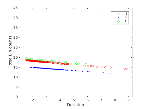
Note in the print out that the dispersion is greater than 1 (1.46), meaning the variance of the data is bigger than expected for a Poisson distribution (where var=mean).
As can be seen in the fitted plot, the blue line is less than the red and green line, and red~=green line. To get all these orderings we need to do post-hoc pairwise tests between the factors, and adjust for multiple comparison. If it was regular ANCOVA, in MATLAB this can be done by acotool and multcompare. Unfortunately multcompare doesn’t work for GLM.
So we do it in R, here are my steps after looking through a bunch of stack exchange posts (last one is on poisson diagnostics).
First write the table in matlab to csv:
>> writetable(ds, '../processedData/lolita_s26_sig072b_bincntData.csv');
In R:
> mydata = read.csv("lolita_s26_sig072b_bincntData.csv")
> mydata$reward_cond = factor(mydata$reward_cond)
> model1 = glm(bincnts ~ durations + reward_cond + durations*reward_cond, family=poisson, data=mydata)
> summary(model1)

Call:
glm(formula = bincnts ~ durations + reward_cond + durations *
    reward_cond, family = poisson, data = mydata)

Deviance Residuals:
    Min       1Q   Median       3Q      Max
-4.1671  -0.8967  -0.1151   0.6881   5.0604

Coefficients:
                       Estimate Std. Error z value Pr(>|z|)
(Intercept)             2.98942    0.03994  74.841  < 2e-16 ***
durations              -0.03960    0.01396  -2.836 0.004568 **
reward_cond0           -0.24969    0.06993  -3.571 0.000356 ***
reward_cond1            0.19174    0.13787   1.391 0.164305
durations:reward_cond0  0.01557    0.02305   0.675 0.499458
durations:reward_cond1 -0.04990    0.04392  -1.136 0.255930
---
Signif. codes:  0 ‘***’ 0.001 ‘**’ 0.01 ‘*’ 0.05 ‘.’ 0.1 ‘ ’ 1

(Dispersion parameter for poisson family taken to be 1)

    Null deviance: 1315.6  on 804  degrees of freedom
Residual deviance: 1165.3  on 799  degrees of freedom
AIC: 4825.8

Number of Fisher Scoring iterations: 4
None of the interaction terms are significant, so we fit a reduced model:
> model1 = glm(bincnts ~ durations + reward_cond, family=poisson, data=mydata)
> summary(model1)

Call:
glm(formula = bincnts ~ durations + reward_cond, family = poisson,
    data = mydata)

Deviance Residuals:
    Min       1Q   Median       3Q      Max
-4.1766  -0.8773  -0.1229   0.7185   5.0664

Coefficients:
             Estimate Std. Error z value Pr(>|z|)
(Intercept)   2.98452    0.03238  92.174  < 2e-16 ***
durations    -0.03773    0.01073  -3.516 0.000438 ***
reward_cond0 -0.20277    0.02003 -10.125  < 2e-16 ***
reward_cond1  0.04229    0.05135   0.823 0.410243
---
Signif. codes:  0 ‘***’ 0.001 ‘**’ 0.01 ‘*’ 0.05 ‘.’ 0.1 ‘ ’ 1

(Dispersion parameter for poisson family taken to be 1)

    Null deviance: 1315.6  on 804  degrees of freedom
Residual deviance: 1167.4  on 801  degrees of freedom
AIC: 4824

Number of Fisher Scoring iterations: 4
This is pretty similar to MATLAB’s results. Before continuing, we can check the dispersion, which is equal to the Residual deviance divided by degrees of freedom. According to this post
> library(AER)
> deviance(model1)/model1$df.residual
[1] 1.457438
> dispersiontest(model1)

    Overdispersion test

data:  model1
z = 5.3538, p-value = 4.306e-08
alternative hypothesis: true dispersion is greater than 1
sample estimates:
dispersion
  1.448394
Again, our dispersion agrees with MATLAB’s estimate. Would this overdispersion invalidate our model fit? According to this CountData document, when this happens, we can adjust our test for overdispersion to use an F test with an empirical scale parameter instead of a chi square test. This is carried out in R by using the family quasipoisson in place of poisson errors. We can do this by fitting the model with a quasipoisson model first, then compare the model fit against a constant model (also quasipoisson) using anova in which we specify test="F":
> model1 = glm(bincnts ~ durations + reward_cond, family=quasipoisson, data=mydata)
> model2 = glm(bincnts ~ 1, family=quasipoisson, data=mydata)
> anova(model1, model2, test="F")
Analysis of Deviance Table

Model 1: bincnts ~ durations + reward_cond
Model 2: bincnts ~ 1
  Resid. Df Resid. Dev Df Deviance      F    Pr(>F)
1       801     1167.4
2       804     1315.6 -3  -148.18 33.931 < 2.2e-16 ***
Still significant! Nice. Another common way to deal with overdispersion is to use a negative-binomial distribution instead. In general, according to Penn State Stat504, overdispersion can be adjusted by using quasi-likelihood function in fitting.
Now multiple comparison – how do I know if the fitted means are significantly different based on reward levels? Use the multcomp R-package’s glht function:
> library(multcomp)
> summary(glht(model1, mcp(reward_cond="Tukey")))

     Simultaneous Tests for General Linear Hypotheses

Multiple Comparisons of Means: Tukey Contrasts


Fit: glm(formula = bincnts ~ durations + reward_cond, family = quasipoisson,
    data = mydata)

Linear Hypotheses:
            Estimate Std. Error z value Pr(>|z|)
0 - -1 == 0 -0.20277    0.02416  -8.392  < 1e-05 ***
1 - -1 == 0  0.04229    0.06196   0.683    0.762
1 - 0 == 0   0.24505    0.06018   4.072 9.42e-05 ***
---
Signif. codes:  0 ‘***’ 0.001 ‘**’ 0.01 ‘*’ 0.05 ‘.’ 0.1 ‘ ’ 1
(Adjusted p values reported -- single-step method)
Here we see the difference between reward_cond=0 and reward_cond=-1, and that between reward_cond=1 and reward_cond==0 are significant, as we suspected looking at the fitted plots. We are fortunate that there is no duration:reward_interactions.
But how would we do multiple comparison when interaction effects are present – i.e. the regression lines have different slopes? We first fit the same data with interaction effects (which we know are not significant):
> model1 = glm(bincnts ~ durations + reward_cond + durations*reward_cond, family=quasipoisson, data=mydata)
> summary(model1)

Call:
glm(formula = bincnts ~ durations + reward_cond + durations *
    reward_cond, family = quasipoisson, data = mydata)

Deviance Residuals:
    Min       1Q   Median       3Q      Max
-4.1671  -0.8967  -0.1151   0.6881   5.0604

Coefficients:
                       Estimate Std. Error t value Pr(>|t|)
(Intercept)             2.98942    0.04822  61.999  < 2e-16 ***
durations              -0.03960    0.01686  -2.349  0.01905 *
reward_cond0           -0.24969    0.08442  -2.958  0.00319 **
reward_cond1            0.19174    0.16643   1.152  0.24963
durations:reward_cond0  0.01557    0.02783   0.559  0.57601
durations:reward_cond1 -0.04990    0.05302  -0.941  0.34693
---
Signif. codes:  0 ‘***’ 0.001 ‘**’ 0.01 ‘*’ 0.05 ‘.’ 0.1 ‘ ’ 1

(Dispersion parameter for quasipoisson family taken to be 1.457184)

    Null deviance: 1315.6  on 804  degrees of freedom
Residual deviance: 1165.3  on 799  degrees of freedom
AIC: NA

Number of Fisher Scoring iterations: 4
Previously, our second argument to glht was mcp(reward_cond="Tukey"). This is telling glht (general linear hypothesis testing) to compare levels of reward_cond and adjust the pvalues with Tukey’s method. When interaction effects are present, we need to define a contrast matrix.
> contrast.matrix = rbind("durations:reward_cond_-1 vs. durations:reward_cond0" = c(0,0,0,0,1,0),
+                         "durations:reward_cond_-1 vs. durations:reward_cond1" = c(0,0,0,0,0,1),
+                         "durations:reward_cond_0  vs. durations:reward_cond1" = c(0,0,0,0,-1,1))
> contrast.matrix
                                                    [,1] [,2] [,3] [,4] [,5]
durations:reward_cond_-1 vs. durations:reward_cond0    0    0    0    0    1
durations:reward_cond_-1 vs. durations:reward_cond1    0    0    0    0    0
durations:reward_cond_0 vs. durations:reward_cond1     0    0    0    0   -1
                                                    [,6]
durations:reward_cond_-1 vs. durations:reward_cond0    0
durations:reward_cond_-1 vs. durations:reward_cond1    1
durations:reward_cond_0 vs. durations:reward_cond1     1
The columns of the contrast matrix corresponds to the rows of the glm coefficients. By default, the base model is selected. So the first row of the contrast matrix will ask for comparison between the base model (durations:reward_cond_-1) and durations:reward_cond0. We give this to glht:
> summary(glht(model1, contrast.matrix))

     Simultaneous Tests for General Linear Hypotheses

Fit: glm(formula = bincnts ~ durations + reward_cond + durations *
    reward_cond, family = quasipoisson, data = mydata)

Linear Hypotheses:
                                                         Estimate Std. Error
durations:reward_cond_-1 vs. durations:reward_cond0 == 0  0.01557    0.02783
durations:reward_cond_-1 vs. durations:reward_cond1 == 0 -0.04990    0.05302
durations:reward_cond_0  vs. durations:reward_cond1 == 0 -0.06547    0.05493
                                                         z value Pr(>|z|)
durations:reward_cond_-1 vs. durations:reward_cond0 == 0   0.559    0.836
durations:reward_cond_-1 vs. durations:reward_cond1 == 0  -0.941    0.603
durations:reward_cond_0  vs. durations:reward_cond1 == 0  -1.192    0.445
(Adjusted p values reported -- single-step method)
And as we already knew, none of the interactions are significant.