Continuing on my quest to have the best unifying intuition about linear algebra, I came across the excellent series Essence of Linear Algebra on YouTube by 3Blue1Brown.

This series really expanded on the intuition behind the fundamental concepts of Linear Algebra by illustrating them geometrically. I have vaguely arrived at the same sort of intuition through thinking about them before, but never this explicitly. My notes are here.

Chapter 1: Vectors, what even are they

Vectors can be visualized geometrically as arrows in 1-D, 2-D, 3-D, …, n-D coordinate system, and can also be represented as a list of numbers (where the numbers represent the coordinate values).

The geometric interpretation here is important to build interpretation and can later be gneralized to more abstract vector spaces.

Chapter 2: Linear combinations, span, and basis vectors

Vectors (arrows, and list of numbers) can form linear combinations, which can involve multiplication by scalars and addition of vectors. Geometrically, multiplication by scalar is equivlaent to scaling the length of a vector by that factor. Vector addition means putting vectors tail to head and find the resulting vector.

Any vectors in 2D space, for example, can be described by linear combinations of a set of basis vectors.

In other words, 2D space are spanned by a set of basis vectors. Usually, the basis vectors are chose to be \([1,0]^T\) and \([0,1]^T\) in 2-D, representing the unit \(\hat{i}\) and \(\hat{j}\) vectors.

As a corollary, if a 3-by-3 matrix \(A\) has linearly-dependent columns, that means its columns does not span the entire 3D-space (spans a plane or a line instead).

Chapter 3: Linear transformations and matrices

Multiplication of a 2-by-1 vector \(v\) by an 2-by-2 matrix \(A\) to yield a new 2-by-1 vector \(u\): \(Au=v\) can be thought of as a linear transformation. In fact, this multiplication can be thought of as transforming the original 2-D coordinate system into a new one, with the caveat the grid lines still have to remain parallel after the transformation (think about a grid getting sheared or rotated).

Specifically, assume the original vector \(v\) is written with basis vectors \(\hat{i}\) and \(\hat{j}\), the columns of \(A\) can be thought of where \(\hat{i}\) and \(\hat{j}\) land in the transformed coordinate system.

Therefore, the matrix-vector multiplication then has the geometric meaning of representing the original vector \(v\) as linear combination of the original basis vectors \(\hat{i}\) and \(\hat{j}\), finding where they map to in the transformed space (indicated by matrix \(A\)), and then yielding \(u\) as the same linear combination of the transformed basis vectors.

This is a very powerful idea – the specific operation of matrix-vector multiplication makes clear sense under this context.

Chapter 4: Matrix multiplication as compositions and Chapter 5: Three-dimensional linear transformations

If a matrix represents a transformation of the coordinate system (e.g. shear, rotation), then multiplication of matrices represent sequences of transformations. For example \(AB\) can represent first shear the coordinate system (\(B\)) then rotate the resulting coordinate system (\(A\)).

This also makes it obvious why matrix multiplication is NOT commutative. Shearing a rotated coordinate system can have different end result as rotating a sheared coordinate system.

Inverse of a matrix \(A\) then represents performing the reverse coordinate system transformation, such that \(A^{-1}A=AA^{-1}\) represents net-zero transformation of the original coordinate system, which is exactly represented by the identity matrix.

Chapter 6: The determinant

This is a really cool idea. In many statistics formulas, there will be a condition that reads like “assuming \(A\) is positive-definite, we multiply by \(A^{-1}\)”. Positive-definite relates to positive determinants. This gave me the sense that determinant represents a matrix analog of real number’s magnitude. But then what does a negative determinant mean?

In the 2D case, if a matrix represents a transformation of the coordinate system, the determinant then represents the area in the transformed coordinate system of a unit area in the original system. Imagine a unit square being stretched, what is the area of the resulting shape – that is the value of the determinant.

Negative determinant would mean a change in the orientation of the resulting shape. Imagine a linear transformation as performing operations to a piece of paper (parallel lines on the paper are preserved through the operations). Matrix with determinant of -1 would correspond to operations that involve flipping the paper. \(\hat{i}\) is originally 90-degrees clockwise from \(\hat{j}\), after flipping the paper (x-y plane), \(\hat{i}\) is now 90-degrees counter clockwise from \(\hat{j}\).

In 3D, determinant then measures the scaling a volume, and negative determinant represent transformations that does not preserve the handed-ness of the basis vectors (i.e. right-hand rule).

If negative determinant represent flipping a 2D paper, then 0 determinant would mean a unit-area becoming zero. Similarly, in 3D, 0 determinant would mean a unit-volume becoming zero. What shape has 0 volume? A plane, a line, and a point. What shape has 0 area? A line and a point.

So if \(det(A)=0\), then we know \(A\) transforms maps vectors into a lower-dimensional space! And that is why positive-definiteness is important, it means a transformation perserves the dimension of the data!

From this intuition, the computation of determinant also makes a bit more sense (at least in the 2D case).

Chapter 7: Inverse matrices, column space and null space

This chapter combines the geometric intuition from before and solving systems of linear equations to explain inverse matrices, column space, and null space.

Inverse matrices

Solving system of linear equations in the form of \(Ax=v\) (wlg, A=3-by-3, x and v are 3-by-1 vectors) can be thought of as what vector \(x\) in 3-D space, after transformation represented by \(A\), become the vector \(v\)?

In this nominal case where \(\|det(A)\|>0\), there exists an inverse \(A^{-1}\) that represents the inverse transformation represented by \(A\), and thus \(x\) can be solved by multiplying \(A^{-1}\) on both sides of the equation.

Intuitively this makes sense – to get the vector pre-transformation, we simply reverse the transformation.

Now suppose \(\|det(A)\|=0\), this means \(A\) maps a 3-D vector onto a lower-dimensional space, which can be a plane, a line, or even a point. In this case, no inverse \(A^{-1}\) exists, because how can you transform these lower-dimensional constructs into 3D space? (Note that in most textbooks, the justification of \(A^{-1}\) exists only when \(det(A)\) is not zero is made on the basis of Gauss-Jordan form, which is not intuitive at all).

Column Space and Null Space

So in the nominal case, each vector in 3D is mapped to a different one in 3D space. Therefore the set of all possible \(v\)’s span the entire 3D space. Therefore the 3D space is the column space of the matrix \(A\). The rank of \(A\) in this case is 3, because the column space is 3-dimensional.

The set of vectors \(x\) that after transformation by \(A\) yield the 0-vector are called the null space of the matrix \(A\).

In cases where \(det(A)=0\), the columns of \(A\) must be linearly dependent, this means its column space is not 3-dimensional, and therefore its rank is less than 3 (and therefore is rank-deficient and not full-rank for a 3-by-3 matrix).

If this rank-deficient \(A\) maps \(x\) onto a plane, then its column space has rank 2. Onto a line – rank 1; Onto a point – rank 0. For a 3-by-3 matrix, 3 minus the rank of the column space is the rank or dimension of the null-space.

Geometrically, this means if a transformation compresses a cube into a plane, then an entire line of points are mapped onto the origin of the resulting plane (imagine a vertical compression of a cube, the entire z-axis is mapped onto the origin and is therefore the null space of this transformation). Similarly, if a cube is compressed into a line, then an entire plane of points are mapped onto the origin of the resulting number line.

Left and Right Inverse

Technically, the inverse \(A^{-1}\) normally talked about refers to the left inverse (\(A^{-1}A=I\)). And the full-rank matrices for which left inverse exist perform a one-to-one transformation of vectors (injective) – each unique vector \(x\) is mapped onto at most one \(v\) vector.

For matrices with more columns than rows, the situation is a bit different. Using our intuition from before treating the columns of matrix as mapping of the original basis vectors into a new coordinate system, consider the matrix \([1, 0; 0, 1; 0, -1]\) mapping a 3D vector. This matrix maps the basis vectors \([1, 0, 0]^T\), \([0, 1, 0]^T\) and \([0, 0, 1]^T\) onto an entire plane, respectively. Therefore each transformed vector can have multiple corresponding vectors in the original 3D space (therefore \(A\) is called surjective).

Consequently, if \(A\) is 2-by-3, there exists a 3-by-2 right-inverse matrix \(B\) such that \(AB=I\), but here \(I\) is 2-by-2. Geometrically, this is saying if we transform a 2D vector onto 3-space (\(B\)), we can recover this 2D vector by another transformation (\(A\)). Thus right-inverse deal with transformations involving dimensional changes.

These explanations, in my opinion, are much more intuitive and easy to remember than the rules and diagram taught in all of the linear algebra courses I have ever taken, including 18.06.

Chapter 8: Nonsquare matrices as transformations between dimensions

This is straight forward applying the idea that the columns of a matrix represent mapping of the basis vectors.

Chapter 9: Dot product and duality

This one is pretty interesting. Dot product represents projection. At the same time, we can think of dot product in 2D, \(v \cdot u\) as a matrix-vector multiplication \(v^T u\). Here we can think of the “matrix” \(v^T\) as a transformation of the basis 2D basis vectors \(\^{i}\) and \(\^{j}\) onto vectors on the number line. Therefore dot-product represents a 2D-to-1D transformation.

This is the idea of vector-transformation duality. Each n-dimensional vector’s transpose represents an N-to-1 dimensional linear transformation.

Chapter 10: Cross products

This one is also not too insightful, perhaps because cross product’s definition as a vector was strongly motivated by physics.

Cross-product of two 2D vectors \(a\) and \(b\) yield a third vector \(c\) perpendicular to both (together obeying right-hand rule) with magnitude equal to the area of the parallelogram formed by the \(a\) and \(b\). Thinking back, cross-product formula involves calculating a type of determinant – which makes sense in terms of the area interpretation of the determinant.

Then the triple product \(\|c\cdot(a\times b)\|\) represents the volume of the parallelpiped formed by \(a\), \(b\), and \(c\).

Chapter 11: Cross products in the light of linear transformations

This one basically explains the triple product by interpreting the dot-product operation (\(c\cdot(\cdot)\)) by the cross-product (\(a\times b\)) as finding a 3D-to-1D linear transformation.

Not too useful.

Chapter 12: Change of basis

This also follows from the idea that a matrix represents mapping of the individual vectors of a coordinate system.

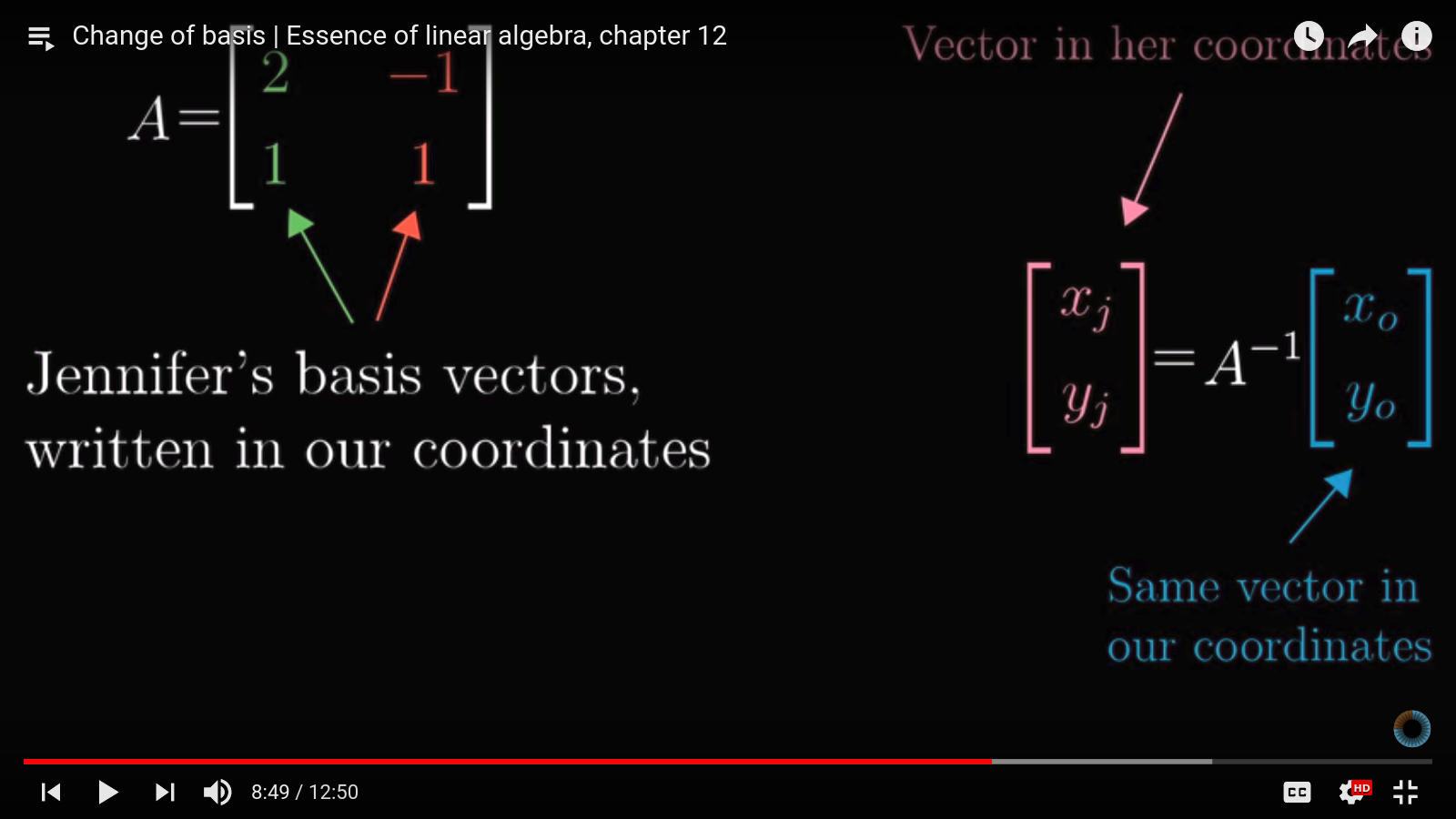
The idea is that coordinate systems are entirely arbitrary. We are used to having \([1,0]^T\) and \([0,1]^T\) as our basis vectors, but they can be a different set entirely. Suppose Jennifer has different basis vectors \([2,1]^T\) and \([-1,1]^T\), how do we represent a vector \([x_0,y_0]^T\) in our coordinate system in Jennifer’s coordinate system?

This is done by a change of basis – by multiplying \([x_0,y_0]^T\) by a matrix whose columns are Jennifer’s basis vectors. This is yet another application of matrix-vector product.

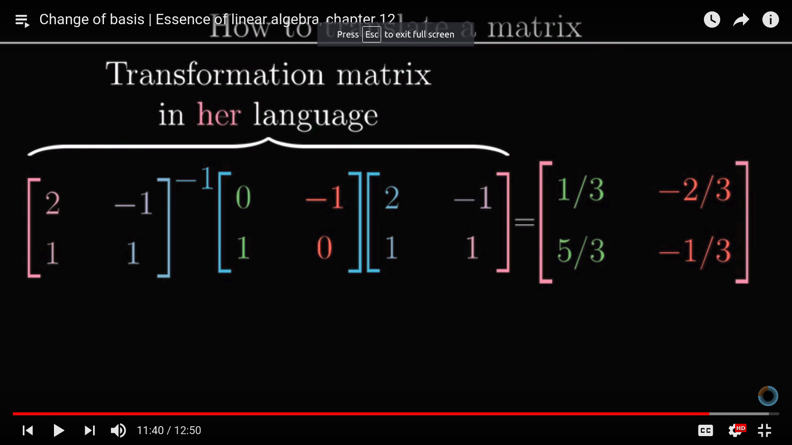
Change of basis can also be applied to translate linear transformations. For example, suppose we want to rotate the vector \(u=[x_1,y_1]^T\) in Jennifer’s coordinate system by 90 degrees and want to find out the result in Jennifer’s coordinate system. It may be tedious to figure out what the 90-degree transformation matrix is in Jennifer’s coordinate system, but it is easily found in our system (\([0,-1;1, 0]\)).

So we can achieve this easily by first transforming \(u\) into our coordinate system by multiplying it by the mapping between Jennfier and our coordinate system. Then apply the 90-degree transformation matrix, then apply the inverse transformation to get back the resulting vector in Jennifer’s system.

This is a powerful idea and relates closely to eigenvectors, PCA, and SVD. SVD especially represents a matrix by a series of coordinate transformations (rotation, scaling and rotation).

Chatper 13: Eigenvector and eigenvalues

This is motivated by the problem \(Av=\lambda v\), where \(v\) are the eigenvectors, and \(\lambda\) are the eigenvalues of the matrix \(A\) (nominally, \(A\) is a square matrix, otherwise we use SVD, but that is beside the point).

The eigenvectors are vectors that, after transformation by \(A\), still point at the same directions as before. A unit vectors before after the transformation may have different length while pointing to the same direction, the change in length is described by the eigenvalue. A negative eigenvalue means the eigenvectors have reversed where it points to after the transformation.

The imagery is suppose we have a square piece of paper/mesh, we pull at the top right and bottom left corners to shear it. A line connecting this two corners will still have the same orientation, though have longer length. Thus this line is an eigenvector, and the eigenvalue will be positive.

However, if a matrix represents rotation, then the determinant will be 0, and the eigenvalues will be imaginary. Imaginary eigenvalues means that a rotation is involved in the transformation.

Chapter 14: Abstract vector spaces

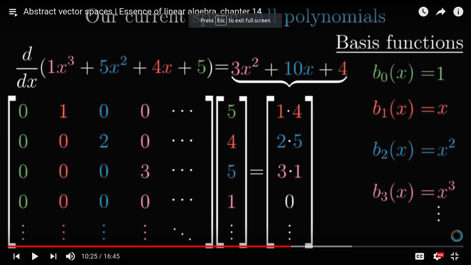
This lesson extrapolate vectors, normally thought of as arrows in 1- to 3-D space and corresponding list of numbers, to any construct that obey the axioms of vector space. Essentially the members of a vector space follow the rule of linear combination (or linearity).

An immediate generalization is thinking of functions as infinite-dimensional vectors (we can add scalar multiples of functions together and the result obey the linearity rule). We can further define linear transformations on these functions, similarly to how matrices are defined on geometric vector spaces.

An example of linear transformation on function is derivative.

This insight is pretty cool and really ties a lot of math and physics concepts together (ex. modeling wavefunctions as vectors in quantum mechanics, eigen-functions as analogs of eigen-vectors).