
The Eighty Five Percent Rule for optimal learning
A practice schedule or learning plan can be very important in skills and knowledge acquisition, thus the saying “perfect practice makes perfect”. I first heard about this work on Andrew Huberman’s podcast on goal setting. The results here are significant, offering insights into both training ML algorithms, as well as biological learners. Furthermore, the analysis techniques are elegant, definitely brushed off some rust here!
Summary
- Examine the role of the difficulty of training on the rate of learning.
- Theoretical result derived for learning algorithms relying on some form of gradient descent, in the context of binary classification.
- Note that gradient descent here is defined as where “parameters of the model are adjusted based on feedback in such a way as to reduce the average error rate over time”. This is pretty general, and both reinforcement learning, stochastic gradient descent, and LMS filtering can be seen as special cases.
- Results show under Gaussian noise distributions, the optimal error rate for training is around 15.87%, or conversely, the optimal training accuracy is about 85%.
- The noise distribution profile is assumed to be fixed, i.e. the noise distribution won’t change from Gaussian to Poisson.
- The 15.87% is derived from the value of normal CDF with value of -1.
- Under different fixed noise distributions, this optimal value can change.
- Training according to fixed error rate yields exponentially faster improvement in precision (proportional to accuracy), compared to fixed difficulty. \(O(\sqrt(t))\) vs. \(O(\sqrt(log(t)))\).
- Theoretical results validated in simulations for perceptrons, 2-layer NN on MNIST dataset, and Law and Gold model of perceptual learning (neurons in MT area making decision about the moving direction of dots with different coherence level, using reinforcement learning rules).
Some background
The problem of optimal error rate pops up in many domains:
- Curriculum learning, or self-paced learning in ML.
- Level design in video games
- Teaching curriculum in education
In education and game design, empirically we know that people are more engaged when the tasks being presented aren’t too easy, and just slightly more difficult. Some call this the optimal conditions for “flow state”.
Problem formulation
The problem formulation is fairly straight-forward, as the case of binary classification and Gaussian noise.
- Agent make decision, represented by a decision variable \(h\), computed as \(h=\Phi(\mathbf{x}, \phi)\), where \(\mathbf{x}\) is the stimulus, and \(\phi\) are the parameters of whatever learning algorithm.
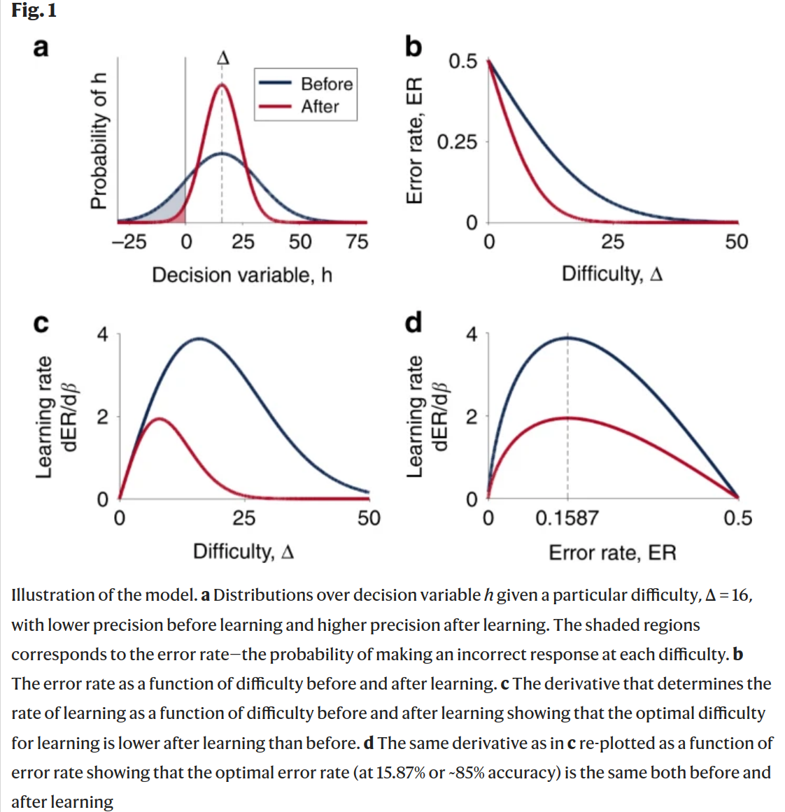
- The decision variable \(h\) is a noisy representation of the true label \(\Delta\): \(h = \Delta + n\), where \(n \approx N(0, \sigma)\).
- If the decision boundary is set at \(h=0\) (see Figure 1A), such that chose A when \(h<0\), B when \(h>0\) and randomly otherwise, then the decision noise leads to error rate of: \[ER = \int_{-\infty}^{0} p(h|\Delta,\sigma)dh=F(-\Delta/\sigma)=F(-\beta\Delta)\].
- p() is Gaussian distribution
- F() is Gaussian CDF
- \(\beta\) is precision, and essentially measures how “peaky” the decision variable distribution is. This can be thought of as the (inverse) accuracy or “skill” of the agent.
- So, the error decreases with both agent skill (\(\beta\)) and ease of problem (\(\Delta\)).
- Learning is essentially an optimization problem, to change \(\phi\) in order to minimize \(ER\). This can be formulated as a general gradient descent problem: \[\frac{d\phi}{dt}=-\eta\nabla_\phi ER\].
- This gradient can be written as \(\nabla_\phi ER = \frac{dER}{d\beta}\nabla_\phi \beta\). And we want to find the optimal difficulty \(\Delta^*\) that maximizes \(\frac{dER}{d\beta}\).
- \(\Delta^*\) turns out to be \(\frac{1}{\beta}\), which gives optimal error rate \(ER^*\approx 0.1587\).
- This is nice, the difficulty level should be proportional to the skill level.
Simulations
Validation of this theory boils down to the following elements:
- How to quantify problem/stimulus difficulty \(\Delta\)?
- How to select problem with the desired difficulty?
- How to adjust target difficulty level to maintain the desired error rate?
- How to measure error rate \(ER\)?
- How to measure skill level?
- Application to perceptron:
- A fully trained teacher perceptron network’s weights \(\mathbf{e}\) are used to calculate the difficulty. The difficulty of a sample is equal to its distance from the decision boundary (higher is less difficult).
- Skill level of the network is \(\cot{\theta}\), where \(\theta\) is the angle between the learner perceptron’s weight vector and the teacher perceptron’s weight vector.
- Error rate is approximately Gaussian and can be determined from the weight vectors of the teacher and learner perceptrons, and the sample vectors.
- Application to two-layer NN:
- Trained teacher network. The absolute value of the teacher network’s sigmoid output is the difficulty of a stimulus.
- Error rate is the accuracy over the past 50 trials (not batch training).
- Skill level is the final performance over the entire MNIST dataset.
- Difficulty level is updated with value proportional to the current and target accuracy level.
- Appliation to Law and Gold model:
- Simulated update rule of 7200 MT neurons according to the orignal reinforcement model.
- Coherence adjusted to hit target accuracy level: implicitly measure difficulty level
- Accuracy/error rate is from past running average
- Final skill level is from applying ensemble on different coherence level stimulus (disabling learning) and fitting logistic regression.
Implications
- Optimal rate is dependent on task (binary vs. multi-class), and noise distribution.
- Batch learning makes things more tricky – depending on agent learning rate.
- Multi-class may require finer grained evaluation of difficulty and problem preseentation (i.e. misclassifying 1v2, or 2v3).
- Not all models follow this framework, e.g. Bayesian learner with perfect memory does not care about example presentation order.
- Can be a good model for optimal use of attention for learning – suppose exerting attention changes the precision \(\beta\), then the benefits of exerting attention is maximized during optimal error rate.