Cortical ensemble adaptation to represent velocity of an artificial actuator controlled by a brain-machine interface

Context Follow-up to the Carmena 2003, Learning to control a brain-machine interface for reaching and grasping by primates paper. In the experiments, monkey first learned to do a target-acquisition task via joystick-control (pole-control), then brain-control was used to control the cursor while the monkey was still allowed to move the pole (brain control with hand movement (BCWH)), and finally the joystick was removed (brain-control without hand movement (BCWOH)). All bin-size=100ms.

Individual cortical neurons do not have a one-to-one relationship to any single motor parameter, and their firing patterns exhibit considerable variablitiy. Precise motor control is achieved through the action of large neuronal ensembles.

The key questions addressed was: How do the neuronal representations of the cursor movement and arm movement of the recorded ensembles change between pole-control, BCWH, and BCWOH?

Method

Implants in M1, PMd, SMA, S1, and PP.

1. Tuning to velocity during pole and brain control. Constructed linear regression model to predict neuronal firing rates based on velocity: \(n(t+\tau)=a(\tau)V_{x}(t)+b(\tau)V_y(t)+c(\tau)+\epsilon(t,\tau)\), where \(t\) is time, \(n(t+\tau)\) is neuronal firing rate at time \(\tau\), \(\tau\) is a time lag. The square root of \(R^2\) for this regression was termed the velocity tuning index (VTI) at \(\tau\). A VTI curve is then constructed for \(\tau\) ranging from [-1,1] second.

2. Preferred direction of a neuron is determined as \(PD(\tau)=arctan(b(\tau)/a(\tau))\).

3. To examine the change in PD between different tasks, correspondence index is defined as: \(C=\frac{90^{\circ}-\overline{|\alpha-\beta|}}{90^{\circ}}\), where \(\alpha\) and \(\beta\) are statistical values calculated from ensembles’ PD measured in degrees for the different tasks. Values of \(C\) approaching zero means no correspondence between the PDs, value approaching 1 means the opposite.

4. Shuffle test to examine how correlations between neurons contribute to tuning properties – destroy correlations between neurons by shifting spike trains of different neurons with repsect to each other by a random interval ranging from 0 to 200s. After shuffling, VTIs are calculated from the regression models in (1). Higher unshuffled VTI would indicate correlated firing between neurons improve tuning characteristics of individual neurons.

5. Straight-line analysis extracted times when trajectories are straight for at least 300ms. VTI were calculated for these times. Directional tuning depth is calculated as the different in average firing rate between the direction of maximum and minimum firing, divided by the SD of the firing rate.

6. Off-line predictions of hand velcocity - is similar to construction of online decoder with: \(V_x(t)=b+\sum^{n}_{\tau=-m}\mathbf{w}(\tau)\mathbf{n}(t+\tau)+\epsilon(t)\)

7. Random neuron dropping: 10min of neuronal population data fit the velocity prediction model. Model then used to predict on a different 10min period. A single neuron is randomly dropped from the population, train then test. This process is repeated until no neurons remained. This entire process (dropping 1 to entire population) is repeated 100 times to yield \(R\) as a function of number of neurons.

Results

1. Hand and robot velocity in pole-control vs. BCWH – More correlated during pole-control (expected), less during BCWH. Ranges of velocity similar. In BCWH, robot moved faster than hand. Ranges of robot velocity similar between BCWH and BCWOH.

2. Neuronal tuning during different modes – Velocity tuning defined as correlation between neuronal rate and velocity. Individual neurons exhibited diversity of tuning patterns:

   • Fig.3: Tuned to both pole-control and brain-control (shown in 3A). VTI higher before instaneous velocity measurement (IVM). VTI for differnet modes significantly different (Kruskal-Wallis ANOVA, Tukey’s multiple comparison). Highest VTI during pole-control. After transitioning to brain control, this neuron retained many features of its original velocity tuning, but also became less tuned to hand movements.

   • Fig.4: Tuned to hand movements. Changes in VTI between different modes are significant. Tuning present during pole-control and BCWH, but vanished in BCWOH. Highest VTI before IVM. Observed lag-dependent PD to both hand and robot velocity. Because of the strong dependency of tuning on the presence of hand movements, this neuron is likely to have been critically involved in generation of descending motor commands.

   • Fig. 5: Tuned to BCWOH.

   Pairwise comparison of pole-control with BCWH and BCWOH (within same sessions) showed in majority of neurons, peak VTI for hand decreased after transitioning to BCWH. In BCWH, the peak VTI for robot is significantly greater than peak VTI for hand for a majority of neurons. Peak VTI during BCWOH was greater than during pole control in \(38\%\) of neurons.

3. Tuning patterns for ensembles

   • Fig.6: Ensemble VTI for different control mode. In majority of neurons, and also average VTI, tuning to hand movement decreased from pole-control to BCWH. VTIs for robot movement is higher pre-IVM, because only bins preceding IVM were used for online prediction, and delay of the robot/cursor introduces a lag. VTI for hand movement peaked closer to IVM than for robot movement. Average VTI similar to M1 VTI due to stronger tuning.

     Occurence of ensemble tuning to robot velocity in BCWOH is not surprising as neural activities controlled robot movement, but it’s not simply a consequence of using the linear model. The shuffled test showed average VTI decreased after the shuffling procedure, indicating role of inter-neuronal correlation in cortical tuning. This corroborates Carmena 2003’s finding that firing of individual neurons is correlated and increase in brain control.

   • Fig 7: Ensemble PD. Generally there was no fixed PD for each neuron and rotated with lag changes (may be due to representation of accelerative and decelerrative forces a la Sergio & Kalaska). In BCWH, PDs for both hand and robot resemble that of pole-control. Correspondence of hand PD between pole-control and BCWH is highest at IVM. For robot PD correspondence is highest 100ms before IVM, which is in agreement with average velocity VTIs. PDs during BCWOH were confined to a narrower angular range and rotated less.

4. Neuronal tuning for selected hand movements.

   • Fig 8: Comparing directional tuning to hand movements in pole-control and BCWH. Both directional tuning depth and VTI w/ respect to hand are less in BCWH. Differences are statistically significant.

5. Offline predictions of hand velocity during pole and brain control. Three prediction curves were made, 1) Using pole-control to train models, then predict pole-control; 2) Train with pole-control, predict BCWH; 3) Train with brain-control, predict BCWH.

   • Fig 9: Prediction quality: (1)>(3)>(2). This decrease in prediction accuracy applies to all lags. Suggests cortical representation of the robot ws optimized at the expense of representation of the animal’s own limb.

Conclusion

1. Principle finding: Once cortical ensemble activity is switched to represent the movements of the artificial actuator, it is less representative of the movement of the animal’s own limb, as evidence by how tuning to hand velocity decreases from pole-control to BCWH.

   • Neuronal tuning to robot movements may be enhanced due to increased correlation between neurons (attention leads to synchrony\(^2\)).

   • Supports evidence that cortical motor areas include cognitive signals as well as limb movements. Limb representation is highly flexible and susceptible to illusions and mental imagery (rubber arm). Neuronal mechanisms underlying adaptive properties\(^1\) may be responsible for cortical ensemble adaptation during the BMI operation.

2. BMI design makes any modulation of neuronal activity translate into movement of the actuator. To interpret it as reflection of new representation of artificial actuators, uses the following evidence:

   • Nonrandomness of actuator movements and behavioral improvements. (Peaking of VTI pre-IVM not neccessarily sufficient because that’s built into prediction algorithms).

   • Increased correlation between neurons during brain control (via Carmena 2003).

   • Decreased tuning to hand velocity in BCWH suggests different representation.

3. Neurons tuned to hand velocity in pole control code for robot velocity in brain-control. How do those neurons’ modulation not lead to hand movements in brain-control? In other words how does the monkey inhibit hand movements during brain control? Suggests activity on the level of ensemble combination changes to accomodate it. The recorded population is small part, may be preferentially assigned weights to control the actuator, whereas the others operate normally. This is the topic of Ganguly and Carmena, 2011.

4. Neuronal ensemble represents robot velocities better during brain control supports optimal feedback control theory – motor system as a stochastic feedback controller that optimizes only motor parameters necessary to achieve task goals (meh).

5. Once the neuronal ensemble starts to control a BMI, imperfections in open-loop model may be compensated by neuronal adaptations to improve control, concurs with (Taylor 2002) using adaptive BMI. Justifies using fixed decoder, and closed-loop decoder calibration stage (CLDA, ReFIT, Schwartz algs).

Further Questions

1. How exactly does the cortical plasticity process help? Very likely features of adaptations depend on requirements of BMI operations. If the task requires both limb movements and BMI operations, what will be the optimal neural system state? It’s possible certain adapation states is only temporary to maintain performance.

   • PDs of many neurons become more similar in BCWOH – may be maladaptive since PD diversity may be needed to improve directional encoding.

   • Shuffling procedures show increased correlations accompanies increased individual neuronal tuning…seems to contradict the previous point.

   • Therefore, neuronal ensemble controlling hte BMI may have been optimizing its performance by trading magnitude of tuning and the diversity of PD, or that increased correlation is only a temporary effect and will decrease with prolonged training (attention in learning stage increases synchrony).

Probably led to Orsborn & Carmena 2014’s task of pressing a button while doing BMI center-out.

\(^1\) – Cortical neurons can encode movement directions regardless of muscle patterns, represent target of movement and movement of the hand-controlled visual marker toward it rather than actual hand trajectory, encode multiple spatial variables, reflect orientation of selective spatial attention, and represent misperceived movements of visual targets.

\(^2\) – Murphy and Fetz, 1992, 1996a,b; Riehle et al., 1997, 2000; Hatsopoulos et al., 1998; Lebedev and Wise, 2000; Baker et al., 2001.

R-Squared, r, and Simple Linear Regression

Linear regression is perhaps the simplest and most common statistical model (very powerful nevertheless), and fits the model of the form:

This model makes some assumptions about the predictor variables, response variables, and their relationship:

1. Weak exogeneity - predictor variables are assumed to be error-free.

2. Linearity - response variables is a lienar combination of the predictor variables.

3. Constant variance - response variables have the same same variance in their errors, regardless of the values of the predictor variables. This is most likely invalid in many applications. Especially so when the data is instationary.

4. Independence of errors - assuming errors of response variables are uncorrelated with each other.

5. Lack of multicollinearity - in the predictors. Regularization can be used to combat this. On the other hand, when there is a lot of data, the collinearity problem is not as significant.

The most common linear regression is fitted with ordinary least-squares (OLS) method, where the sum of the squares of the differenceces between the observed responses in the dataset and those predicted by the model is minimized.

Two very common metrics associated with OLS linear regression is coefficient-of-determination \(R^2\), and correlation coefficient, specifically Pearson correlation coefficient \(r\).

The first measures how much variance is explained by the regression, and is calculated by \(1-\frac{SS_{res}}{SS_{tot}}\). The second measures the the lienar dependence between the response and predictor variables. Both have value between 0 and 1. Say we fit linear regression and want to check how good that model is, we can get the predicted value \(\mathbf{\hat y}=\mathbf{X}\beta\) and check the \(\mathbf{R^2}\) and \(\mathbf{r}\) values between \(\mathbf{y}\) and \(\mathbf{\hat y}\). When a linear regression is fit using OLS, then the \(R^2=r^2\).

However, if two vectors are linearly related but not fit using OLS regression, then they can have high \(r\) but negative \(R^2\). In MATLAB:

1
2
3
4
5
6
7
8
9
10
11
12
13
14
15
16
17
18
19
20
21
22
23
24
25
26
>> a = rand(100,1);
>> b = rand(100,1);
>> corr(a,b)

ans =

    0.0537

>> compute_R_square(a,b)

ans =

   -0.7875

>> c = a + rand(100,1);
>> corr(a,c)

ans =

    0.7010

>> compute_R_square(a,c)

ans =

   -2.8239

Even though a and c above are clearly linearly related, their \(R^2\) value is negative. This is because the \(1-\frac{SS_{res}}{SS_{tot}}\) definition assumes c is generated from an OLS regression.

According to Wikipedia,

Important cases where the computational definition of R2 can yield negative values, depending on the definition used, arise where the predictions that are being compared to the corresponding outcomes have not been derived from a model-fitting procedure using those data, and where linear regression is conducted without including an intercept. Additionally, negative values of R2 may occur when fitting non-linear functions to data.[5] In cases where negative values arise, the mean of the data provides a better fit to the outcomes than do the fitted function values, according to this particular criterion

This point really tripped me up when I was checking my decoder’s performance. Briefly, I fit a Wiener filter to training data, apply on testing data, and then obtain the \(R^2\) and \(r\) between the predicted and actual response of the testing data. I expected \(R^2=r^2\). However, \(R^2\) was negative and its magnitude was not related to \(r\) at all – precisely for this reason.

In the case of evaluating decoder performance then, we can instead:

1. Fit a regression between \(\mathbf{y}\) and \(\mathbf{y_{pred}}\), then check the \(R^2\) of that regression. Note that when there is a lot of data, regardless of how weak the correlation is between them, the fit will be statistically significant. So while the value of \(R^2\) is useful, its pvalue is not as useful.

2. Correlation coefficient \(r\). However it is susceptible to outliers when there is not much data. This has been my go-to metric for evaluating neural tuning (as accepted in the field) and decoder performance.

3. Signal-to-Noise (SNR) ratio. As Li et al., 2009 pointed out, \(r\) is scale and translational invariant, this means a vector \([1,2,3,4,5]\) and \([2,3,4,5,6]\) will have \(r=1\), which does not capture this offset.

SNR is calculated as \(\frac{var}{mse}\) (often converted to dB) where \(var\) is the sample variance \(y\), and \(mse\) is the mean squared error of \(y_{pred}\). This then measures how \(y_{pred}\) ‘tracks’ \(y\), as desired.

Neural correlates of decision variables in parietal cortex

Motivation

Sensory-motor reflex has been tacitly accepted by many older physiologists as an appropriate model for describing the neural processes that underlie complex behavior. More recent findings (in the 1990s) indicate that, at least in some cases, the neural events that connect sensation and movement may involve processes other than classical relfexive mechanisms and these data suppport theoretical approaches that have challenged reflex models directly.

Researchers outside physiology have long argued (since 1960s) for richer models of the sensory-motor process. These models invok3 the explicit representation of a class of decision variables, which carry information about the environment, are extracted in advance of response selection, aid in the interpretatin or processing of sensory data and are a prerquisite for rational decision making.

This paper describes a formal economic-mathematical approach for the physiological studey o fthe senosry-motor process/decision-making, in the lateral intra-parietal (LIP) area of the macaque brain.

Caveats

1. Expectation of reward magnitude result in neural modulations in the LIP. LIP is known to translate visual signals into eye-movement commands.

2. The same neurons are sensitive to expected gain and outcome probability of an action. Also correlates with subjective estimate of the gain associated with different actions.

3. These indicate neural basis of reward expectation.

Decision-Making Framework

The rational decision maker makes decision based on two environmental variables: the gain expected to result from an action, and the probability that the expected gain will be realized. The decision maker aims to maximize the expected reward.

Neurobiological models of the processes that connect sensation and action almost never propose the explicit representation of decision variables by the nervous system. Authors propose a framework containing

1. Current sensory data - reflect the observer’s best estimate of the current state of the salient elements of the environment.

2. Stored representation of environmental contingencies - represent the chooser’s assumptions about current environmental contingencies, detailing how an action affects the chooser.

This is a Bayesian framework.

Sensory-Motor integration in LIP

In a previous experiment, the authors concluded that visual attention can be treated as conceptually separable from other elements of the decision-making process, and that activity in LIP does not participate in sensory-attentional processing but is correlated with either outcome continguencies, gain functions, decision outputs or motor planning.

Experiments

1. Cue saccade trials: a change in the color of a centrally located fixation stimulus instructed subjects to make one of two possible eye-movement responses in order to receive a juice reward. Before the color change, the rewarded movement was ambiguous. The successive trials, the volume of juice delivered for each instructed response (expected gain), or the probability that each possible response would be instructed (outcome probability) are varied.

   Goal is to test whether any LIP spike rates correlate to variations in these decision variables.

2. Animals were rewarded for choosing either of two possible eye-movement responses. In subsequent trials, varied the gain that could be expected from each possible response. The frequency with which the animal chose each response is then an estimate of the subjective value of each option.

   Goal is to test whether any LIP activity variation correlates with the subjective estimate of decision variable.

Analysis

Experiment 1

For each condition: 1) keeping outcome probability fixed while varying expected gain, and 2) keeping expected gain fixed while varying outcome probability, a trial is divded into 6 200ms epochs. The activity during these epochs are then used to calculate regressions of the following variables:

1. Outcome probability.
2. Expected gain.
3. Type of movement made (up or down saccade).
4. Amplitude of saccade.
5. Average velocity of saccade.
6. Latency of saccade.

Multiple regression were done for each epoch, percentage of recorded neurons that show significant correlations between firing rate and the decision variables were calculated.

Average slope of regression against either decision variables were taken as a measure of correlation. The same regressio slopes were calculated for type of movement made as well.

For both expected gain and outcome probability, the regression slopes were significantly greater than 0, and greater than that for type of movement during early and late visual intervals, and decay during late-cue and movement. The opposite is seen for type of movement regression slopes.

Experiment 2

Similar analysis is done to evaluate neural correlate of subjective estimate of reward. Results show activity level correlates with the perceived gain associated with the target location within the neuron’s receptive field. The time evolution of the regression slopes show a similar decay as before.

Consistent with Herrnstein’s matching law for choice behavior, there was a linear relationship between the proportion of trials on which the animal chose the target inside the response field and the proportion of total juice available for gaze shifts to that target.

Animal’s estimate of the relative value of the two choices is correlated with the activation of intraparietal neurons.

Discussions

1. It would seem obvious that there are neural correlates for decision variables, rather than the traditional sensory-motor reflex decision-making framework. But this may be solely in the context of investigating sensory areas..probably have to read Sherrington to know how he reached that conclusion.

2. The data in this paper can be hard to reconcile with traditional sensory-attentional models, which would attribute modulations in the activity of visually responsive neurons to changes in the behavior relevance of visual stimuli, which would then argue that the author’s manipulations of expected gain and outcome probably merely altered the visual activity of intraparietal neurons. Explainations include:

   • Previous work show intraparietal neurons are insensitive to changes in the behavioral relevance of either presented stimulus when it is not the target of a saccade.

   • Experiment 2 showed that intraparietal neuron activity was modulated by changes in the estimated value of each response during the fixation intervals BEFORE the onset of response targets.

3. Modulations by decision variables early in trial. Late in trial more strongly modulated by movement plan. Suggests intraparietal cortex lies close to the motor output stages of the sensory-deicsion-motor process. Prefrontal cortex perhaps has reprsentation of decision variables throughout the trial.

Classifier performance in primary somatosensory cortex towards implementation of a reinforcement learning based brain machine interface, submitted to Southern Biomedical Engineering Conference, 2016.

In the theme of RL-based BMI decoder, this paper evaluates classifiers for identifying the reinforcing signal (or ERS according to Millan). Evaluates the ability of several common classifiers to detect impending reward delivery within S1 cortex during a grip force match to sample task performed by monkeys.

Methods

1. Monkey trained to grip right hand to hold and match a visually displayed target.

2. PETHs from S1 generated, from 1) aligning with timing of visual cue denoting the impending result of trial (reward delivered or withheld), 2) aligning with timing of trial outcome (reward delievery or withold).

   PETH time extended 500ms after stimulus of interest using a 100ms bin width. (So only 500ms total signal, 5-bin vector samples).

3. Dimension-reduction of PETH via PCA. Use only the first 2 PCs, feed into classifiers including:

   • Naive Bayes
   • Nearest Neighbor (didn’t specify how many k…or just one neighbor..)
   • Linear SVM
   • Adaboost
   • Quadratic Discriminant Analysis (QDA)
   • LDA

   Trained on 82 trials, tested on 55 trials. Goal is to determine if a trial is rewarding or non-rewarding.

Results

1. For all classifiers, post-cue accuracy higher than post-reward accuracy. Consistent with previous work (Marsh 2015) showing the presence of conditioned stimuli in reward prediction tasks shift rerward modulated activity in the brain to the earliest stimulus predictive of impending reward delivery.

2. NN performs the best out of all classifiers. But based on the sample size (55 trials) and the performance figures, not significantly better.

Takeaways

Results are good, but should have more controlled experiments to eliminate confounds…could be seeing an effect of attention level.

Also, still limited to discrete actions.

Parietal Lobe: From Action Organization to Intention Understanding

Inferior parietal lobule (IPL) neurons were studied when monkeys performed motor acts embedded in different actions, and when they observed similar acts done by an experimenter. Most IPL neurons coding a specific act (e.g. grasping) showed markedly different activiations depending on contexts (e.g. grasping for eating or for placing).

Many motor IPL neurons also discharged during the observation of acts done by others. The context-dependence also applied to when these actions were observed.

These neurons fired during the observation of an act, before the beginning of the subsequent acts specifying the action - thus these neurons not only code the observed motor acts but also allow the observer to understand the agent’s intentions.

Posterial parietal cortex has traditionally been considered as the association cortex. Besides “putting together” different sensory modalities, also

1. Codes motor actions
2. Provides the representations of these motor actions with specific sensory information.

Experiment

Set 1

Investigates neuron selectivity during actioin performance:

1. Monkey starts from a fixed position, reache for and grasp a piece of food located in front of it and brigh the food to mouth.
2. Monkey reach for and grasp an object, and place it in a box on the table.
3. Monkey reach for and grasp an object, and place it into a container near its mouth.

Most observed neurons discharged differentially with respect to context.

Control for confounds:

1. Grasp an identical piece of food in both conditions - rewarded with the same piece of food in situation 2.
2. Situation 3 aims to determine if arm kinematics determined the different firing behavior - turns out to be pretty much identical to situation 2.
3. Force exerted grasping - mechanical device that could hold the objects with two different strengths used, no change in neuron selectivity.

Set 2

Study 41 mirror neurons that discharge both during grapsing observation and grasping execution, in an experiment where the monkey observed an experimenter performing those actions.

Results:

1. Some neurons are selective for grasping to eat, others for grasping to place - most have the same specificity as when the monkey performed those actions.
2. Most neurons have the same selectivity regardless of whether the grasped object is food or solid. Some discharged more strongly in the placing conditions when the grasped object was food.

The authors suggest that while counter-intuitive, this should makes sense since motor acts are not related to one another independent of the global aim of the action but appear to form prewired intentional chains in which each motor act is faciliatted by the previously executed one. This reminds me of Churchland and Shenoy’s theory about action planning as a trajectory in the Null-Space.

Consequences

The authors suggest that the monkey’s decision on what to do with the object is undoubtedly made before the onset of the grasping movement. The action intentionis set before the beinning of the movements and is already reflected in the first motor act. This motor reflectioin of action intention and the chained motor organization of IPL neurons have profound consequences on […] understanding the intention of others.

While I can see where he reaches this conclusion, and it would nicely explain why passive observation training for BMI works (even though mostly M1 and S1 neurons are recorded), but this explanation would make more sense if most of the difference in discharge rate happens BEFORE the monkey physically grasp the object/food…

It has been generally accepted that mirror neurons allow the observing individual to understand the goal of the observed motor act. The authors’ interpretation then deduces that because the monkey knows the outcome of the motor act it executes, it recognizes the goal of the motor act done by another individual when this act triggers the same set of neurons that are active during the execution of that act.

Applications to BMI

This paper suggests mirror neurons as a mechanism for evaluation of intention, it also suggests that depending on context and object, a simple grasp action may be coded differently. Thus a BMI arm trained on passive observation of grasping an object to place might not work well when the user tries to grasp a food to eat. This is similar to when the Schwarz 10-DOF arm encountered, when the human subject had trouble grasping object. The problem only went away when the training was done in a virtual space.

Errare machinale est: the use of error-related potentials in braine-machine interfaces

This review focuses on electrophysiological correlates of error recognition in human brain, in the context of human EEG. Millan calls this error-related potentials, ErrPs. It has been proposed to use these signals to improve BMI, in the form of training BMI decoder via reinforcement learning.

Error-related brain activity

Early reports in EEG date back to early 1990’s (Falkenstein et al., 1991; Gehring et al., 1993). Showed a characteristic EEG event-related potential elicited after subjects commited errors in a speed repsonse choice task, characterized by a negative potential deflection, termed the error-related negativity, appearing over fronto-central scalp areas at about 50-100ms after a subject’s erroneous response. The negative copmonent is followed by a centro-parietal positive deflection.

Modulations of this latter component have been linked to the subject’s awareness of the error. ERN amplitude seems to be modulated by the importance of erros in the given task. These signals have been shown to be quite reliable over time and across diferent tasks.

Very encouraging for reinforcement-learning based schemes.

fMRI, EEG-based source localization, and intra-cranial recordings suggest that the fronto-central ERP modulations commonly involve the medial-frontal cortex, specifically the anterior cingulate cortex (ACC). This is consistent with ACC being involved in reward-anticipation and decision-making.

Error-related potentials for BMI

Ferrez and Millan 2008: 2-class motor-imagery bsaed BMI controlling a cursor moving in discrete steps – showed ERPs elicited after each command could be decoded as corresponding to the error or correct condition with an accuracy of about 80%. Only 5 subjects, but encouraging.

The ErrP classifiers maintained the same performance when tested several months after calibration - relatively stable signal form. Seemed to be mainly related to a general error-monitoring process, not task-dependent.

Possible Confounds (in EEG studies):

1. Eye movement contamination: Need to make sure location or movement of target stimuli are balanced.
2. Observed potentials are more related to the rarrity of the erroneous events (?)
3. Attential level: subjects tend to have smaller ErrP amplitude when simply monitoring the device than when they are controling it – requires efficient calibration methods.

Error-Driven Learning

Trials in which the decoder performed correctly, as classified by ErrP can be incorporated into a learning set that can be then used to perform online retraining of the motor imagery (MI) classifier. Rather discrete, but good architecture.

Binary ErrP decoding can be affected substantially by false positive rate (i.e. correct BMI actions misclassified as errors). Solution is to use methods relying on probabilistic error signals, taking into account of the reliability of the ErrP decoder.

Millan has used ErrP to improve his shared-control BMI systems.

A learning-based approach to artificial sensory feedback leads to optimal integration

Motivation

Maximally precise movements are achieved by combining estimates of limb or target positiion from multiple sensory modalities, weighting each by its relative reliability. Current BMI relies on visual feedback alone, and would be hard to achieve fluid and precise natural movements. Artificial proprioception may improve performance of neuroprosthetics.

Goal

Artificial proprioception should be able to:

1. Provide sufficient information to alow competent performance in the absence of other sensory inputs.
2. Permit multisensory integration with vision to reduce movement variability when both signnals are available. Implemented via multichannel intracortical microstimulation. Different from most other works that take a biomimetic approach. It focuses not on reproducing natural patterns of activity but instead on taking advantage of the natural mechanisms of sensorimotor learning and plasiticity.

Hypothesize spatiotemporal correlations between a visual signal and novel artificial signal in a behavioral context would be sufficient for a monkey to learn to integrate the new modality.

Approach

Monkey looks at a screen, trying to move to an invisible target. The movement vector is the vector between the monkey’s current hand position and the invisible target.

1. Visual feedback: The movement vector is translated to random moving-dot flow field. The coherence of the dot-field is the percentage of dots moving in the same direction. So 100% coherence dot-field would have the dots moving in the same direction as the movement vector.
2. ICMS: 96-channels array is implanted. 8 electrodes were stimulated on. During feedback, the movement vector is decomposed into 8 components in direction equally spaced around a circle, each corresponding to a stimulating electrode. Higher relative frequency on an electrode means greater component of the movement vector in that direction. Common frequency scaling factor corresponds to movement vector distance.

Experiments inluded:

1. Learning the task with only visual feedback, with different coherence to demonstrate performance differences due to changing sensory cue precision.
2. Learning the task with only ICMS feedback. Trained by providing ICMS during visual task to teach monkey to associate the spatial relationship. No changing coherence.
3. Performing the task with both.

Metrics:

1. Percent trials correct
2. Number of movement segments - small is better. Movement segment found by assuming sub-movements have bell-hsaped velocity profiles – identify submovements by threshold crossings of the radio velocity plot of a trajectory.
3. Normalized movement time: by the distance to target.
4. Noramlized path length: Normalized the integrated path length by the distance from start to target.
5. Mean and Variance of the initial angle: Used to compare initial movement direction and movement vector.
6. Distance estimation: Assess the monkey’s ability to estimate target distance from ICMS by regressing initial movement distance against target distance for ICMS-only trials, excluding trials for which the first movement segment was not the longest.

Evaluating Sensory Integration

Minimum variance integration, which is supposed to the optimal integration, predicts that in VIS+ICMS condition, as the visual coherence increases from 0% to 100%, the animals should transition from relying primarily on the ICMS cue to primarily on the visual cue – under the model of minimum variance integration, each sensory cue should be wieghted inversely proportional to its variance.

Results

1. Monkey learns all three tasks.
2. VIS+ICMS outperforms VIS only for visual coherence less than 50%.
3. Optimal (minimum variance integration) integration of the two sensory modalities observed.

And only 8 electrodes!!

I can apply linear algebra, but often forget/confuse the spatial representations.

A good resource is Gilbert Strang’s essay. I remember him talking about this when I took 18.06, but he was old at that point, and I barely went to class. So I didn’t retain much. This notes of his still retains his stream of consciousness style, but the two diagrams summarizes it well, and is useful to often go back and make sure I still understand it.

The first one shows the relationship between the four subspaces of a matrix \(A\). The second one adds in the relationship between the orthonormal basis of the subspaces.

Strang concludes:

Finally, the eigenvectors of \(A\) lie in its column space and nullspace, not a natural pair. The dimensions of the spaces add to \(n\), but the spaces are not orthogonal and they could even coincide. The better picture is the orthogonal one that leads to the SVD.

The first assertion is illuminating. Eigenvectors \(v\) are defined such that \(Av=\lambda v\). Suppose \(A\) is \(M\times N\), then \(v\) must be \(M\times 1\), therefore eigenvectors only work when \(M=N\). On the other hand, in SVD, we have \(A=U\Sigma V^T\) and

• \(Av_i=\sigma_i u_i\) for \(i=1,...,r\), where \(r\) is the rank of column and row space.

  \(u_i\) are the basis for the column space (left singular vectors), \(v_i\) are the basis for the row space (right singular vectors).

  The dimensions for this equation matches because the column space and row space are more natural pair.

• \(Av_i=0\), \(A^Tu_i=0\), for \(i>r\).

  \(v_i\) are the eigenvectors of the null space of \(A^T\),

  \(u_i\) are the eigenvectors of the null space of \(A\).

  They also match up similarly (Figure 2).

• In \(Ax=b\), \(x\) is in the row space, \(b\) is in the column space.
• If \(Ax=0\), then \(x\) is in the null space (kernel) of A, and is orthogonal complement of the row space of A, \(C(A^T)\).
• In \(A^Tx=b\), \(x\) is in the column space, \(b\) is in the row space.
• If \(A^Tx=0\), then \(x\) is in the cokernel of A, and is orthogonal complement of the column space of A, \(C(A)\).

Relationship with PCA ***

PCA Algorithm Inputs: The centered data matrix \(X\) and \(k\gt1\).

1. Compute the SVD of \(X\): \([U,\Gamma,V]=svd(X)\).
2. Let \(V_k=[\mathbf{v}_1,...,\mathbf{v}_k]\) be the first \(k\) columns of \(V\).
3. The PCA-feature matrix and the reconstructed data are: \(Z=XV_k, \hat{X}=XV_kV_k^T\).

So in PCA, the rows of the data matrix are the observations, and the columns are in the original coordinate system. The principle components are then the eigenvectors of the row space. We can do PCA in MATLAB with pca or manually with svd:

1
2
3
4
5
6
7
8
9
10
11
12
13
14
15
16
17
18
19
20
21
% PCA test
a = rand(100,1);
b = 5*a+rand(100,1);

data = [a, b];  % rows are observations
plot(a,b, '.');


% PCA results
% coeffs=PC in original coordinate[PxP], 
% scores=observation in PC-space [NxP], 
% latent=variance explained [Px1]
[coeffs, score, latent] = pca(data);
hold on;
plot(score(:,1), score(:,2), 'r.');

% SVD results
centeredData = bsxfun(@minus, data, mean(data,1));
[U, S, V] = svd(centeredData);
svd_score = centeredData*V;
plot(svd_score(:,1), svd_score(:,2), 'g.');

The results shown below. Blue is original data, green/red are the PCA results, they overlap exactly. Note that MATLAB’s pca by default centers the data.

Projection into subspace (e.g. Kaufman 2014, Cortical activity in the null space, Even-Chen 2017, Neurally-driven error detectors) ***

Suppose we have a trial-averaged neural activity matrix \(A\) of size \(N\times T\), where \(N\) is number of neurons, and \(T\) is number of time bins.

In online BMI experiment, a linear decoder maps the neural activity vector \(n_t\) of size \(N\times 1\) to kinematics \(v_t\) of size \(2\times 1\) via the equation \(v_t = w n_t\), where \(w\) is of size \(2\times N\).

Kaufman describes the output-potent neural activities as collection of \(n_t\) such that \(v_t\) is not null. Therefore the output-potent subspace of \(n_t\) is the rowspace of \(w\). Similarly, the output-null subspace is the null space of \(w\).

By projecting the activity matrix \(A\) into these subspaces, we can get an idea of how much variance in the neural activities can be accounted for the modulation to control actuator kinematics:

1. Use SVD on \(w=U\Sigma V^T\) to get its row and null space, defined by the first \(r\) columns of \(V\) (call it \(w_{potent}\)), and the last \(N-r\) columsn of \(V\) (call it \(w_{null}\)), respectively, where \(r\) is the rank of \(w\).
2. Left multiply \(A\) by these subspaces (defined by the those columns) to get \(A_{potent}\) and \(A_{null}\).
3. The variance of \(A\) explained by projection into the subspaces is obtained by first subtracting each row’s mean from each matrix, then taking the L2 norm of the entire matrix (Frobenius norm of the matrix).

Philip Sabes’ Linear Algebra notes

Wiener Filter

Wiener filter is used to produce an estimate of a target random process by LTI filtering of an observed noisy process, assuming known stationary siganl and noise spectra. This is done by minimizing the mean square error (MSE) between the estimated random process and the desired process.

Wiener filter is one of the first decoding algorithms used with success in BMI, used by Wessberg in 2000.

Derivations of Wiener filter are all over the place.

1. Many papers and classes refer to Haykin’s Adaptive Filter Theory, a terrible book, in terms of setting the motivation, presenting intuition, and the horrible typesetting.

2. MIT’s 6.011 notes on Wiener Filter has a good treatment of DT noncausal Wiener filter derivation, and includes some practical examples. Its treatment on Causual Wiener Filter, which is probably the most important regarding real-time processing, is mathematical and really obscures the intuition – we reach this equation from completing the square and using Parseval’s theorem, without mentioning the consquences in the time domain. My notes

3. Max Kamenetsky’s EE264 notes gives the best derivation and numerical examples of the subject for practical application, even though only DT is considered. It might get taken down, so extra copy [here](/reading_list/assets/wienerFilter.pdf}. Introducing the causual form of Wiener filter using input whitening method developed by Shannon and Bode fits into the general framework of Wiener filter nicely.

Wiener Filter Derivation Summary

1. Both the input \(\mathbf{x}\) (observation of the target process) and output \(\mathbf{y}\)(estimate of the target process \(\mathbf{d}\), after filtering) are random processes.

2. Derive expression for cross-correlation between input and output.

3. Derive expression for the MSE between the output and the target process.

4. Minimize expression and obtain the transfer function in terms of \(\mathbf{S_{xx}}\) and \(\mathbf{S_{xd}}\), where \(\mathbf{S}\) are Z or Laplace transforms of the cross-correlations.

This looks strangely similar to a linear regression. Not surprisingly, it is known to statisticians as the multivariate linear regression.

Kalman Filter

In Wiener Filter, it is assumed that both the input and target processes are WSS. If not, one may assume local stationarity and conduct the filtering. However, nearly two decades after Wiener’s work, Rudolf Kalman developed the Kalman filter, which is the optimu mean square linear filter for nonstationary processes (evolving under a certain state space model) AND stationary ones (converging in steady state to Wiener filter).

Two good sources on Kalman Filter:

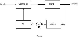
1. Dan Simon’s article describes the intuition and practical implementation of KF, specifically in an embedded control context. The KF should be coupled with a controller when the sensor reading is unreliable – it filters out the sensor noise. My notes

   

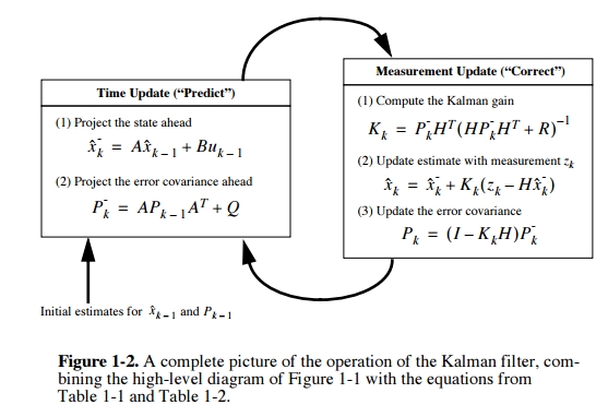
2. Greg Welch and Gary Bishop’s An Introduction to the Kalman Filter. Presents just the right amount of math in the derivation of the KF. My notes

3. Update (12/9/2021): New best Kalman Filter derivation, by Thacker and Lacey. Full memo, Different link.

The general framework of the Kalman filter is (using notation from Welch and Bishop):

The first equation is the state model. \(x_k\) denotes the state of a system, this could be the velocity or position of a vehicle, or the desired velocity or position of a cursor in BMI experiment. \(A\) is the transition matrix – describes how the state will transition depending on past states. \(u_k\) is the input to the system. \(B\) describes how the inputs are coupled into the state. \(w_k\) is the process noise.

The second equation is the observation model - it describes what kind of measurements we can observe from a system with some state. \(z_k\) is the measurement, it could be the speedometer reading of the car (velocity would be the state in this case), or it could be neural firing rates in BMI (kinematics would be the state). \(H\) is the observation matrix (tuning model in BMI applications). \(v_k\) is the measurement or sensor noise.

One caveat is that both \(w\) and \(v\) are assumed to be Gaussian with zero mean.

The central insight with Kalman filter is that, depending on whether the process noise or sensor noise dominates, we weigh the state model and observation model differently in their contributions to compute the new underlying state, resulting in a posteriori state estimate \[\hat{x_k}=\hat{x_k}^- + K_k(z_k-H\hat{x}_k^-)\] Note the subscript \(_k\) denotes at each discrete time step.

The first term \(\hat{x_k}^-\) is the contribution from the state model - it is the a priori state estimate based on the state model only. The second term is the contribution from the observation model - given the a posteriori state estimate.

Note a priori denotes a state estimate at a given time state \(k\) to use only knowledge of the process prior to step \(k\). a posteriori denotes a state estimate that also uses the measurement at step \(k\), \(z_k\).

\(K\) is the Kalman gain, the derivation of which is the most mathematically involved step. The derivation involves the definition of:

1. \(P_K^-\): the a priori estimate error covariance \[P_k^-=E[e_k^-e_k^{-T}]=E[(x_k-\hat{x_k}^-)(x_k-\hat{x_k}^-)]\].
2. \(P_K\): the a posteriori estimate error covariance \[P_k=E[e_ke_k^T]=E[(x_k-\hat{x_k})(x_k-\hat{x_k})^T]\].

To derive \(K\), we want to minimze the a posteriori state estimate \(P_K\), which makes intuitive sense. A good estimate of the state is one that minimizes the variance of the estimation error. A bunch of math later, we obtain \[K_k=P_k^-H^T(HP_k^-H^T+R)^{-1}\].

Looking at the a posteriori state estimate equation, we can see that

1. If the sensor noise is extremely low, i.e. \(R\rightarrow 0\), then we should trust the sensor reading, and \(\hat{x_k}\) should just be \(H^{-1}z_k\). This is indeed the case as \(\lim_{R_k\to 0}K_k=H^{-1}\).

2. If the process noise is extremely low, i.e. \(Q\rightarrow 0\), then we should trust the state model on how the state should change, thus \(\hat{x_k}\) should just equal to the a priori state estimate \(\hat{x_k}^-\). This is indeed the case as \(\lim_{P_k^-\to0}K_k=0\).

In implementation, KF operates by alternating between the prediction phase and a correct phase. The prediction phase projects the state based on the state model. The correction phase updates the estimate from the predictioin phase by the measurement and observation model. Operation is recursive and efficient.

Thus the KF is a generalization of the Wiener filter when the input and reference processes are non-stationary. This is done by estimating the state, tracking the changing statistics in the non-stationary process. This tracking is enabled by the incorporating the measurements taken.

KF is superior to Wiener Filter also because

1. There are less parameters to be fitted.
2. The movement and observation models are decoupled, providing more flexibility in system design.

Extended Kalman Filter (EKF)

The default KF addresses the general problem of trying to estimate the state \(x\) goverend by a linear stochastic model. However, when the state and/or observation model is nonlinear, the KF needs to linearize about the current mean and covariance.

Therefore, \(A\), \(B\), \(H\), \(w\) and \(v\) need to be replaced by the Jacobians linearized at the current mean and covariance. The math is different, but the architecture is the same.

Unscented Kalman Filter (UKF)

UKF is used a better implementation of KF for nonlinear state and observation model. Why use UKF when we can use EKF?

According to wikipedia, whe the state and observation models

are highly non-linear, the extended Kalman filter can give particularly poor performance. This is because the covariance is propagated through linearization of the underlying non-linear model. The unscented Kalman filter (UKF) uses a deterministic sampling technique known as the unscented transform to pick a minimal set of sample points (called sigma points) around the mean. These sigma points are then propagated through the non-linear functions, from which the mean and covariance of the estimate are then recovered. The result is a filter which more accurately captures the true mean and covariance.

In Zheng Li’s 2009 paper, Unscented Kalman Filter for Brain-Machine Interfaces, he applies the UKF to BMI. The keypoints were:

1. UKF allows nonlinear neuron tuning model – this is a nonlinear observation model. In the paper, the tuning model is quadratic and describes the tuning better than a linear one.

2. UKF also allow a nonlinear movement model – nonlinear state model.

3. The movement model was made to be of degree-n, meaning that the state equation is no longer a function of the previous state, but of the previous n states. Incorporating this “movement history” acts as smoothing for the output kinematics.

The number of sigma points was chosen to be \(2d+1\), where \(d=4n\) is the dimension of the state space. If \(n=10\), then \(d=40\), big state space.

The name unscented is pretty dumb and provides no clue to how it modifies the KF.

Adaptive UKF

As a follow up to the 2009 paper, Li published Adaptive UKF. This algorithm modifies on the n-degree UKF by including

Bayesian regression self-training method for updating the parameters of an unscented Kalman filter decoder. This novel paradigm uses the decoder’s output to periodically update the decoder’s neuronal tuning model in a Bayesian linear regression.

So, the tuning model/observation matrix \(H\) is updated online periodically. Great for modeling the plasticity associated non-stationarity.

ReFIT-KF

Last september I went through Caltech’s Learning from Data course offered through EdX. Went through all the lectures and homework except for the final exam.

Finally got around to finish it this week, after re-reading some forgotten materials. All the code written for the problem sets are here. Some notes:

VC Dimension and Generalization

One of the most emphasized point in the course, is how to estimate the generalization performance of an algorithm. VC-Dimension can be used as a preliminary measure of an algorithm’s generalization performance. A more complex hypothesis is more likely to overfit, and given the same amount of training data, may lead to worse generalization. When possible, using simpler hypothesis set is better. Otherwise, use regularization.

Linear Regression

Simple, not very sexy, but surprisingly powerful in many applications. Combined with nonlinear transforms can solve many classes of problems. We have many techniques that can solve linear problems. So in general, want to try to reduce problems into this class.

Validation

Cross-validation, especially leave-one-out, is an unbiased estimator of the out of sample error \(E_{out}\).

Use validation for model selection, including parameters for regularization.

SVM

Very powerful technique. Motivation is simple - finding a hyperplane that separats two classes of data with the greatest margin from the separation plane to the closest points of each class. Solving the equations become a quadratic programming problem of minimizing the norm of the weights of the plane (which is inversely proportional to the margin width), subject to the all points being classified correctly (in hard-margin SVM).

This original formulation is called the primal problem.

The same problem can be formulated into a LaGarange Multiplier problem, with an additional multiplier parameter \(\alpha_i\) for each data point. This problem then requires the minimizing over the weights, after maximizing over the multiplier \(\alpha\)s. Under the KKT conditions (or vice versa), we can switch the order to maximizing over the multipliers after minimizing over the weights. This allows us to write expressions for the weights in terms of \(\alpha\) after doing the minimization (by taking the partial derivatives of the expression).

Finally, we reach another Quadratic-Programming problem, where the objective is over \(\alpha\)s, subjective to constraints from the weights’ minimization.

The advantages of this Dual Problem is that the data points are present in the expression in terms of inner products – allowing us to use the kernel trick, which is a computationally efficient way of doing nonlinear transformation to higher-order (even infinite) dimensions.

One of the coolest thing about SVM is that, according to strict VC-dimension analysis, after nonlinear transformation of the data points into infinite dimensions via the kernel trick, \(E_{out}\) should be unbounded. However, because SVM searches for hyperplane with the fattest separation margin, the effective VC-dimension is significantly reduced, and thus \(E_{out}\) is under control.

RBF

RBF network classifiers places a RBF on each training data point, and then classifies test points by summing those RBF values at the test point.

Since this is prohibitive when data set is big, we can instead pick K representative points, by finding the centroid of K clusters (via clustering algorithm). Therefore, the classification problem is transformed into a linear regression problem, where the basis are the RBF centered around the cluster centers.

SVM with RBF kernel still outperforms the regular-RBF network classifiers most of the time. Why do we use it? I can imagine doing unsupervised learning: have a cluster of data points with no labels, but simply use clustering + RBF to derive K labels and assign them to new samples.

Results of the comparison in terms of the metrics given in the metrics post.

Right click to open plots in a new window to see better

Victor Purpura

In this plot, the x-axis is the acceptable time shift we can shift a spike in the recording to match one in the reference, and equal to \(1/q\), where \(q\) is the shift-cost in the original VP formulation.

When the acceptable time shift is small, VP is a measure of the number of non-coincident spikes. When the shift is large, it is more a measure of difference in spike counts.

As expected, the performance is much worse when SNR is low. As expected, Plexon performs well on the VP metric across all timescales. RHD has very close performance, except in the 10ms scale. This is most likely due to the onboard spike-sorting uses only 0.5ms window rather than the full 1ms window used in Plexon, resulting in missed spikes or shifted spike times. I expect the difference between plexon and RHD to decrease with shorter spike duration/features.

RHA has the worst performance, and this is especially apparent for low SNR recordings. The difference of the performance difference between RHA and RHD is most likely RHA’s use of AGC. When SNR is low, AGC also amplifies the noise level - therefore a burst in noise may result in amplitude similar to a spike. This is also apparent when trying to align the RHA and reference waveforms prior to metric comparison - with simple peakfinding it is impossible to align the signals properly when SNR=1dB. More advanced frequency-domain techniques may be needed. Therefore, the cyan RHA curve should be counted as an outlier.

The mean and standard deviation plot confirms the above. At time scales greater than 10ms, plexon and RHD have very close performance over different SNRs.

van Rossum

The x-axis is the \(\tau\) parameter used in the exponential kernel. As \(\tau\) increases, the metric is supposed to measure non-coincident spikes to difference in spike counts and firing rate.

I would expect the curves to show the same trend as that in the VP distance. But instead it shows the opposite trend. Further, the results don’t agree with the other tests…therefore I must conclude even the corrected Paiva formula is incorrect..?

Schreiber

The x-axis is the \(\sigma\) parameter used in the Gaussian kernel. As \(\sigma\) increases, the metric measures the non-coincident spikes to difference in spike counts and firing rates. The curves show the expected shape. And again, at time scale greater than 10ms, all three systems have simlar performance.

Binned Distance

The x-axis is the bin size used in calculating the binned distance. The order of the curves are almost the same as that in the VP-distance. Again, Plexon performs the best for small time scale, all three systems converge in performrance with increasing bin size.

The mean curve shows the convergence for binned distance is a lot steeper than that for VP-distance. This is really good news, as most of our decoding algorithms use binned firing rates. It shows for bin size \(>=25ms\), the wireless systems have performarnce very close to Plexon.

Finally, the order of performrance is again \(plexon>RHD>RHA\).

Some computation problems/notes I encountered while implementing the metrics. Code

Victor Purpura Distance

Victor-Purpura’s MATLAB implementation, adapted from the Seller algorithm of DNA sequence matching, while having \(O(N_i N_j)\) performance runs pretty slow.

For a test comparison of two spike trains, one with 8418 spike times and the other with 9782 spike times, it takes around 75 seconds. A bit too long. On Victor’s page, there are a few other Matlab implementations, but only deal with parallelizing calculations with different cost of shifting a spike. The mex function has weird usage. So I tried translating the algorithm into Julia and calling it from Matlab. The result is spkd_qpara.jl:

Pretty straight forward. Importing my spike time vectors into Julia and running the function, it takes about 1.07 seconds, a significant speed-up. However, most of my analysis, plotting, and data are in Matlab, so I would like to call Julia from Matlab. This functionality is provided by jlcall.

Configuration through running jlconfig as instructed in the README was smooth, except for the message:

Warning: Unable to save path to file ‘/usr/local/MATLAB/R2015a/toolbox/local/pathdef.m’. You can save your path to a different location by calling SAVEPATH with an input argument that specifies the full path. For MATLAB to use that path in future sessions, save the path to ‘pathdef.m’ in your MATLAB startup folder.

In savepath (line 169) In jlconfig (line 100)

Warning most likely related to my machine.

Using any methods from Jl.m, however, was not. I received the error: Invalid MEX-file '/home/allenyin/.julia/v0.4/jlcall/m/jlcall.mexa64': libjulia.so: cannot open shared object file: No such file or directory.

So it seems Matlab cannot find the libjulia.so. This is documented jlcall’s bug list.

Simple fix is as suggested in the message thread: in Matlab do setenv('LD_RUN_PATH', [getenv('LD_RUN_PATH'), ':', '/usr/lib/x86_64-linux-gnu/julia') before running the jlconfig script. The path given is the location of the so file.

Now to call victorD from Matlab, do:

1
2
Jl.include(`spkd_qpara.jl');
Jl.call('victorD', spikeTimes1, spikeTimes2, 200);

The second call takes 1.41 seconds.

Van Rossum Distance

Paiva 2009 derived a computational effective estimator with order \(O(N_iN_j)\) for the VR-distance:

\(d_{vR}(S_i,S_j)=\frac{1}{2}[\sum_{m=1}^{N_i}\sum_{m=1}^{N_i}L_{\tau}(t_m^i-t_n^i)+\sum_{m=1}^{N_j}\sum_{m=2}^{N_j}L_{\tau}(t_m^j-t_n^j)]+\sum_{m=1}^{N_i}\sum_{n=1}^{N_j}L_{\tau}(t_m^i-t_n^j)\),

where \(L_{\tau}(\cdot)=exp(-abs(\cdot)/\tau)\) is the Laplacian kernel. However, this formula is wrong. By inspection we can see that this distance will never be 0 since it is a sum of exponentials. Further sample calculation for distance between less similar spike trains may even yield smaller distance! These problems can be corrected by changing the sign of the last summation term. Unfortunately, this typo occurs in (Paiva et al., 2007) as well as Paiva’s PhD thesis. However, as I can’t derive the formula myself (there must be some autocorrelation trick I’m missing), I don’t trust it very much.

It is nevertheless, a much more efficient estimator than the naive way of taking the distance between convolved spike trains, and does not depend on time discretization.

Thomas Kreuz has multiple van Rossum Matlab code posted on his website, but they don’t work when \(\tau<20ms\).

Schreiber Distance

This dissimilarity measure also have a data-effective method of \(O(N_iN_j)\), given in Paiva 2010.

Generating Test Signals

Signals were generated using Leslie Smith and Nhamoinesu Mtetwa’s Noisy Spike Generator MATLAB Software v1.1 (NSG) using makeReferenceSignals.m.

Sampling rate was set to 31250Hz since that is the sample rate of the wireless headstages. This frequency is greater than the maximum Plexon ADC frequency of 20,000Hz, but offline analysis may simply use interpolation.

Notes on using this toolbox:

1. The main script generatenoisysamples.m outputs a final signal that includes noise from uncorrelated spike noise, correlated spike noise, and Gaussian noise. The NoiseSNR only sets the Gaussian noise level. As this validation is on recording quality, not spike sorting algorithm, I modified that script to not include the uncorrelated and correlated spike noise in the final output.

2. While the manual of the toolbox claims that the spike duration can be changed by changing the T_Delta_Integrate and N_Delta_integrate parameters (spike duration is T_Delta_Integrate X N_Delta_Integrate). However, changing these parameters simply changes how many samples it takes from a pre-generated template file. These template files were generated by the author and the script used was not available. Regardless, the default spike duration of ~1.8ms, while longer than most motor cortex spikes we encounter, can still be sorted and detected by all three systems teseted.

Aligning Reference with Recording

After the reference signals are generated, they are converted to .wav files with Fs=31250Hz. All audio signals (including those with two distinct spikes firing) are available on soundcloud. The audio signals then goes through the Plexon headstage test board, to which the wireless and plexon headstage may connect.

As mentioned in Validation of signal quality I, since the reference signal and the recording cannot be started and stopped at exactly the same time, some alignment needed to be done before applying the spike train measurements.

The reference and recording are aligned in the start by aligning the peak of the first spike in the reference with that of the recording. I use the recorded analog waveform, rather than the recorded spike times for alignment because the first spike may not be detected, and it’s easier to examine the alignment quality visually from the analog waveforms.

The first spike peak of the reference signal is easily found by doing peak-finding on a 5ms window after the first spike-time (which is known). The spike times generated by NSG marks the beginning of a spike, not the peak.

When SNR is high, peak-finding on the recording can also find the peak of the first recorded spike pretty easily. But with lower SNR, the noise level gets higher and the MinPeakHeight parameter of MATLAB’s findpeaks() must be adjusted so that a noise peak is not being mistaken for a signal peak. Of course, it’s not always possible to align two signals, contributing to bad spike train comparison. The best MinPeakHeight for found this way for each recorded signal is in compare_signals.m. The script checkAlignment.m helps with that.

For the end of the recording signal - sometimes when I don’t stop the input audio signal in time, extra signal is recorded. Thus after alignment, I cut the recording to within 102 seconds of the alignment start.

While recent work such as A wireless transmission neural interface system for unconstrained non-human primates focuses on the how transmitted analog waveform compares to that recorded by wired commerical systems, our validation goal is somewhat different.

While our wireless system operates also streams full analog waveforms, the focus is on onboard spike sorting and reporting spikes. Therefore, the most important measure is how the reported spike trains compares with that of the ground truth and that sorted/measured by commercial wired systems. Thus spike-train analysis is conducted here.

Systems compared:

1. RHA-headstage with resistor-set RHA-Intan filtering, AGC, and four stages of IIR digital filtering. Final bandwidth is 500Hz-6.7kHz or 150Hz-10kHz.

2. RHD-headstage with onchip-resistor-set RHD-Intan filtering (1Hz-10kHz), manually set fixed gain (Q7.8 ranges -128:0.5:127.5), and two stages of IIR digital filtering. Final bandwidth is 250Hz-9kHz.

   I observed it’s much easier to do spike sorting keeping the Intan onboard bandpass filter to have wide bandwidth, so the displayed waveform is not too distorted. The IIR filters can apply sufficient filtering to remove low and high frequency noise to expose the key spike features. But having access to the signal prior to IIR can be very helpful for sorting, especially when SNR is low. Finally, changing from AGC to user-set fixed gain seems to yield much cleaner signals since AGC amplifies noise as well, making it very difficult to sort under low SNR. Downside is it’s neccessary to check the templates often to make sure the previously set gain is enough.

3. Plexon (old Harveybox..), standard spike filtering options. Waveform uses 20kHz sampling rate.

All three systems use manual PCA spike sorting. While the actual sorting interface has a time window of 1ms, the headstages use only templates that are 0.5ms long to sort spikes onboard.

Measures used:

To compare spike train performance, I referred to A comparison of binless spike train measures; Paiva, Park, Principe 2010 for a review and comparison of these measures. Very useful despite an amateur error with one of the formulas.

1. Victor-Purpura Distance(VP)

   The first binless distance measure proposed in the literature. Defines the distance between two spike trains in terms of the minimum cost of transforming one spike train into the other by means of just three basic operations: spike insertion (cost 1), spike deletion (cost 1), and shifting a spike by some interval by \(\Delta t\)(cost \(q\|\Delta t\|\)). The cost per time unit, \(q\) sets the time scale of the analysis. For \(q=0\) the distance is equal to the difference in spike counts, while for large \(q\) the distance is linearly proportional with the number of non-coincident spikes, as it becomes more favorable to delete and reinsert all non-coincident spikes rather than shifting them (cost 2 in this instance). Thus, by increasing the cost, the distance is transformed from a rate distance to a temporal distance. Note that the cost is inversely proportional to the acceptable time shift between two spikes.

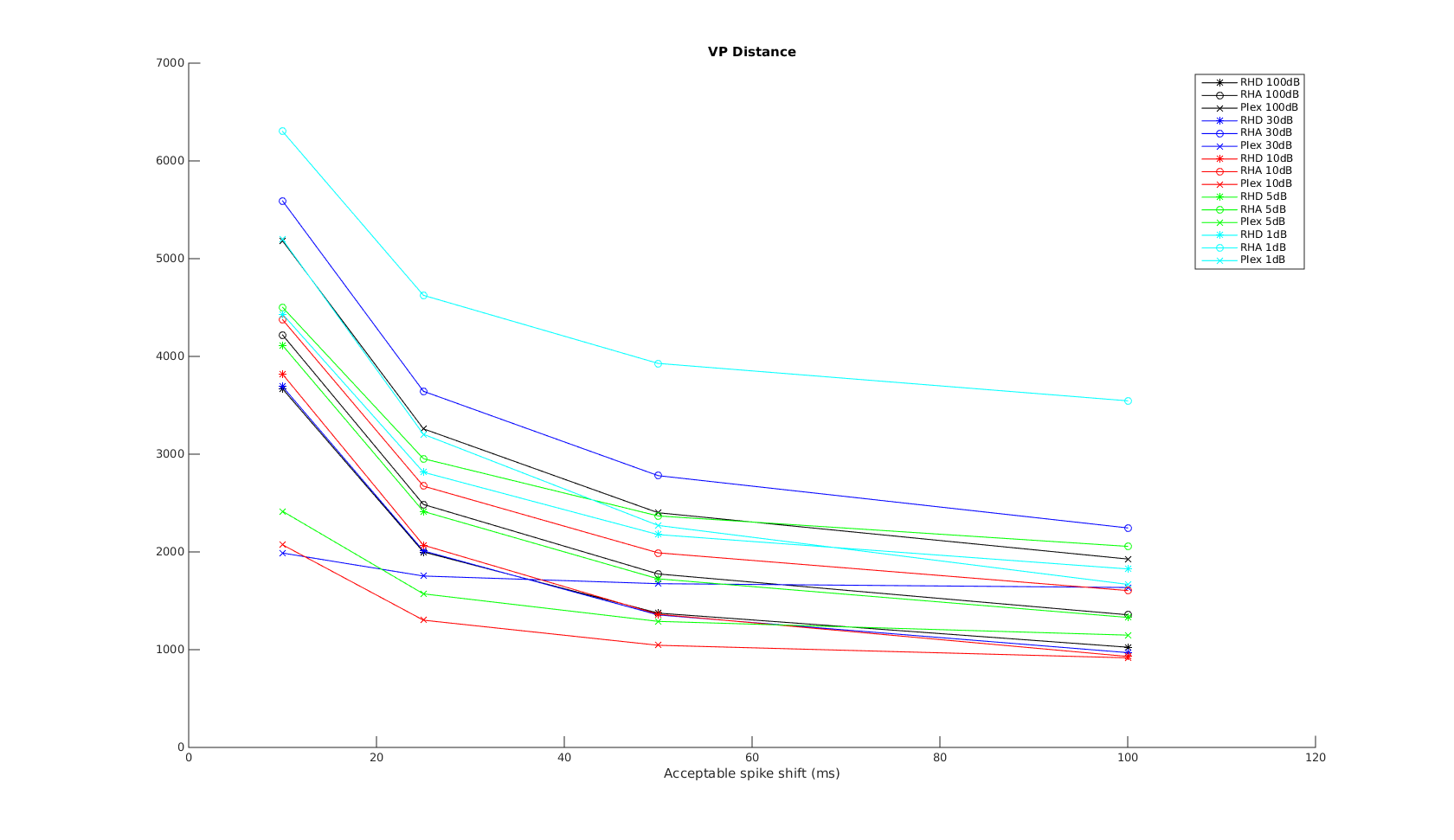
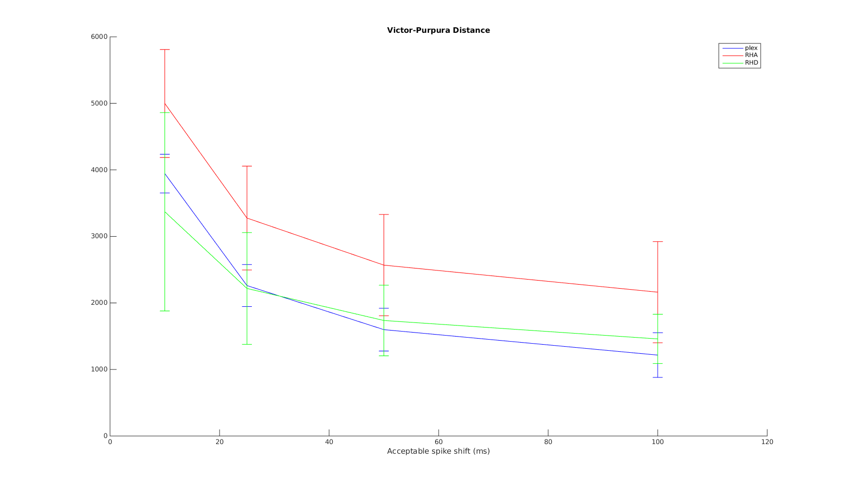
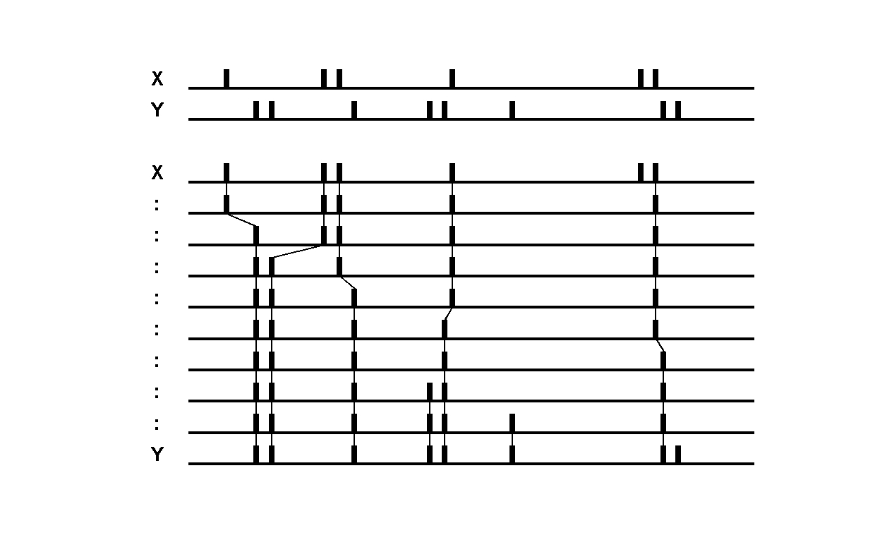
   Victor-Purpura spike train distance. Two spike trains X and Y and a path of basic operations (spike deletion, spike insertion, and spike shift) transforming one into the other. (Victor and Purpura, 1996).

2. Van Rossum Distance(VR)

   Similar to the VP-distance, VR distance utilizes the full resolution of the spike times. The VR distance is the Euclidean distance between exponentially filtered spike trains.

   A spike train \(S_i\) is defined as \(S_i(t)=\sum_{m=1}^{N_i} \delta(t-t_m^i)\), where \(\{t_m^i:m=1,...,N_i\}\) are the spike times.

   After convolving this spike train with a causal decaying exponential function \(h(t)=exp(-t/\tau)u(t)\), we get the filtered spike train \(f_i(t)=\sum_{m=1}^{N_i} h(t-t_m^i)\). The Van Rossum distance between two spike trains \(S_i\) and \(S_j\) is the Euclidean distance:

   \[d_{vR}(S_i,S_j)=\frac{1}{\tau}\int_0^{\infty} [f_i(t)-f_j(t)]^2 dt\]

   For VR, the parameter \(\tau\) sets the time scale, which can be though of as inversely related to VP’s \(q\) parameter. The metric acts as a count of non-coincident spikes (temporal relationship) to a difference in spike count (spike rates) as the kernel size \(\tau\) is increased. This is opposite of what happens to VP distance as \(q\) is increased.

3. Schreiber-correlation dissimilarity

   The Schreiber dissimilarity based on the correlation measure defined in terms of Gaussian-filterd spike trains. In this approach, the filtered spike train \(S_i\) becomes \(g_i(t)=\sum_{m=1}^{Ni} G_{\sigma/\sqrt{2}}(t-t_m^i)\), where \(G_{\sigma/\sqrt{2}}(t)=exp(-t^2/\sigma^2)\) is the Gaussian kernel. The role of \(\sigma\) here is similar to \(\tau\) in Van Rossum distance, and is inversely related to \(q\) in VP distance. Assuming a discrete-time implementation of the measure, then the filtered spike trains can be seen as vectors, for which the usual dot product can be used. Therefore a correlation like dissimilarity measure can be derived:

   \[d_{CS}=1-r(S_i,S_j)=1-\frac{\vec{g_i}\cdot\vec{g_j}}{\|\vec{g_i}\|\|\vec{g_j}\|}\]

   This metric is always betweeen 0 and 1, and can be thought of as a measure of the angle between the two filtered spike trains. Note that this quantity is not a strict distance metric because it does not fulfill the triangel inequality. Chicharro 2011 suggests that this measure’s applicability to estimate reliability is limited because of the individual normalization of spike trains, which renders the measure sensitive only to similarities in the temporal modulation of the individaul rate profiles but neglects differences in the absolute spike count.

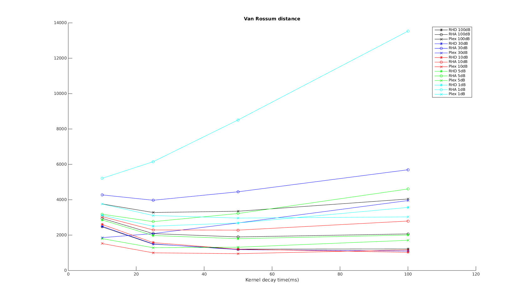
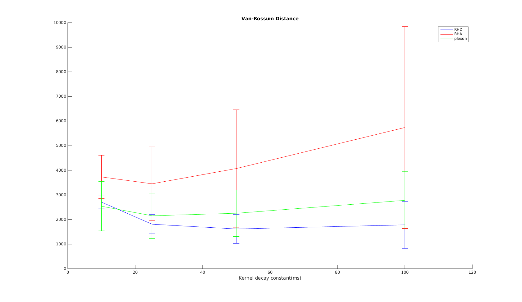
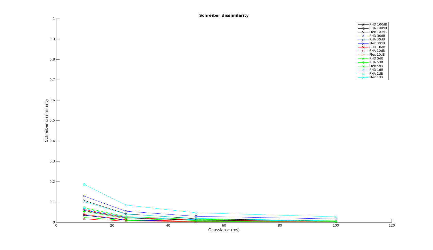
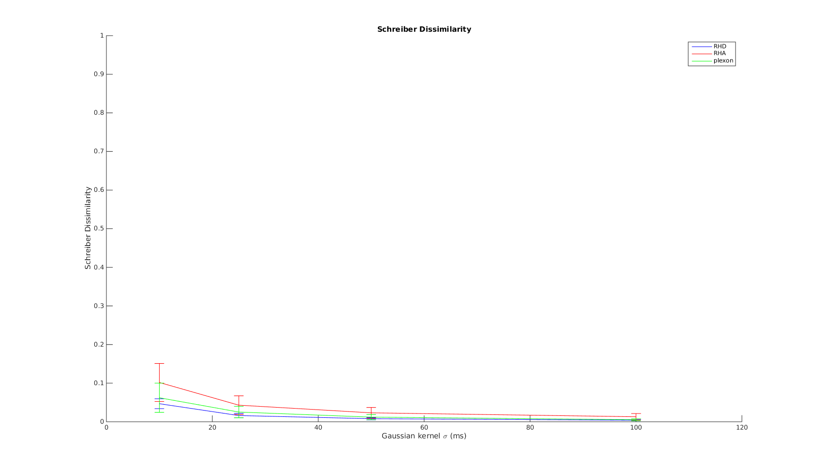
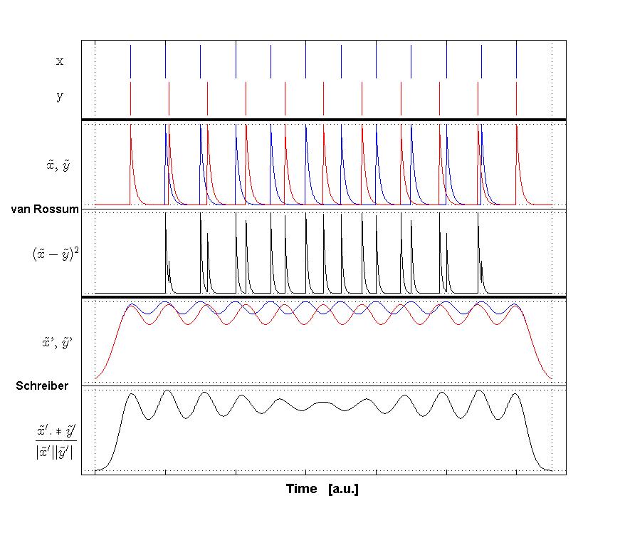
   Van Rossum spike train distance and Schreiber et al. similarity measure. Figure from (van Rossum, 2001) and (Schreiber et al., 2003)

4. Binned distance (\(d_B\))

   While both Paiva2010 and Chicharro2011 recommends not using a binned method to measure spike train similarity, it is more directly related to BMI methods. The binned distance is simply the sum of the absolute value of the two binned spike trains, which would require us to compare spike trains of the same length.

Notes

According to simulation tests conducted by Paiva 2009, none of the above measures performs the best or consistently when measuring different aspects of spike-train similarity, including 1) discriminating different firing rate; 2) discriminating changing firing rate; 3) Spike train synchrony. In the end, Paiva concludes:

1. VP and van Rossume distances perform better discriminating constant firing rate.
2. Schreiber and binned-distance perform better discriminating synchrony.
3. All measures performed similar in discriminating instantaneous firing rates.

Ideally, validation should tell us exactly what percentage of detected spikes are true positives, and how many spikes we have missed. But that requires probabilistic calculation (e.g. is a spike false positive, or just a shifted spike) that is difficult, I settle for these metrics that are well established and are relevant for BMI – the firing rates are usually binned and normalized prior to decoding, which is sensitive to time scales. There are other time-scale independent spiket rain distances such as event synchronization (Quiroga 2002), SPIKE synchronization (Kreuz 2015), ISI-distance (Kreuz 2007a), and SPIKE-distance (Kreuz 2013), but they are in my opinion harder to interpret.

After finishing work on the wireless headstage, it occured to me that no comprehensive validation has been done to confirm spike-sorting and signal quality of the wireless headstages. So I’m conducting a semi-rigourous testing of the RHA-headstage, RHD-headstage, agains the Plexon recordings. This paper on a Blackrock-based wireless system testing has been useful.

First part, I want to examine the signal quality of the streamed raw waveform. The basic setup is:

1. Generate a neural signal of known length, save this as an audio signal with sampling frequency Fs=31250Hz. This is chosen because the headstage’s sampling frequency is 31250Hz.
2. An extra button was added to gtkclient so that as sson as it starts recording the incoming data from the headstages, it also launches VLC to play that audio signal.
3. Keep recording until the end of the audio signal.

The recorded signal can then be plotted and analyzed for signal quality.

Note that the command to VLC to play the audio signal is launched from within gtkclient through the system() command. As a result, the headstage is not actually recording that audio signal until after a short VLC initialization delay. This is consistently around 0.5 seconds, as measured by VLC log.

To compare the recorded signal quality against the reference signal, the first test is by visual inspection. Since the recorded signal is a simulated neural signal, this becomes – do the spike features (sharp peaks and valleys) line up? A more quantitative measure is the cross-correlation between the reference and recorded signals, but the resulting value is a bit harder to interpret.

For the visual test, as a result of the VLC delay, we must shift the recorded waveform to align with the beginning of the reference signal. See below for original signals and aligned signals. Blue is reference, red is recording. The signals are 100 seconds long, with dt=1/31250s.

Note the short red segment in the top plot in the beginning, that signals the absence of audio signal.

We can inspect the aligned waveform (by aligning the peak of the first spikes in each signal). In the beginning (shown below), we can see the spike features align fairly well. The squiggles in the red signal are due to noise and filtering artifacts, which are ok in this case but poses the SNR lower limit with which we can distinguish neural signals.

Around the middle of the signal (around 45.82s), we see the signals are no longer aligned. Rough inspections show the red recorded signal has developed a lead over the blue signal - the recording signal has shifted to the left of the reference signal. The three labeled red peaks correspond to the three labeled blue peaks. This is confirmed by the relative time between the labled peaks.

We can further make a table of where the corresponding labeled peaks occur within their respective signals, in terms of sample number:

|Recording samp#       | Ref samp#            | Diff in samp#    | Diff in ms 
-----------------------|----------------------|------------------|------------
1432167                | 1432972              | 805              | 25.76      
1432707                | 1433515              | 808              | 25.856     
1433025                | 1433830              | 805              | 25.76      

the last column is calculated by dividing the Diff in samp# by 31250Hz to obtain the lead in seconds, then to ms.

Near the end of the signal (around 96.056s), the lead becomes even greater, as shown below.

And the corresponding table of labeled peak locations:

|Recording samp#       | Ref samp#            | Diff in samp#    | Diff in ms 
-----------------------|----------------------|------------------|------------
3001750                | 3003284              | 1534             | 49.088    
3002059                | 3003620              | 1561             | 49.952
3002839                | 3004374              | 1535             | 49.12      
3003072                | 3004612              | 1540             | 49.28

The developing lead in sample numbers between the two recorded signals are most likely due to loss of packets from the wireless headstage. Each packet contains new waveform samples, and if they are lost, our recorded signal will be effectively shortened from the reference signal, resulting in this lead. And since the number of lost packets can only increase, this lead will simply increase with time.

While this is a problem when we are doing offline analysis of the recorded signals, it should not be a huge deal in terms of real-time BMI applications where we care about the instantaneous firing rate – as long as we dont lose too many packets. As Tim has stated in his thesis:

1 in 3176 packets were rejected on average; assuming one bit error per packet, this equates to a bit error rate (BER) of 1.23e-6, or approximately one bit error per second. Efforts to reduce this have not been successful, but the system works acceptably presently.

This matches what I have seen empirically, and comparisons against Plexon. As long as the BER is on the order of 1e-6, then packet loss should not affect performance too much.

The current software keeps track of the total number of lost packets. It might be of interest to find how this changes through time. The previous tables seems to suggest that the number of samples lost increase linearly with time, which supports my hypothesis that the shift is due to last packets. To get a better idea, however, I would want to perform that same analysis around different time points along the signal, probably within a sliding window. Matlab’s findpeaks() function can extract the positions of the different peaks within the signals, but matching them would be more difficult. While it is relatively easy via visual inspection, it seems to me to be NP-hard…what’s an efficient algorithm to do this?

Update - Perhaps a sliding window of seller’s algorithm to match the ‘edit distance’ of the peaks would answer the question, but that’s not too important for our goal of validation.

Conventional electrodes used in BMI include the Utah Array, Michigan Array, and the Duke microwire array, which have been used in most BMI work so far.

I compile here a list of unconventional electrodes that I come across.

1. Multifunctional fibers for simultaneous optical, electrical and chemical interrogation of neural circuits in vivo - Polina Anikeeva, MIT

2. Syringe-injectable electronics - Charles Lieber, Harvard

3. Stent-electrode - Thomas Oxley, University of Melbourne.

   Measures only LFP up to 200Hz.

Just finished reading The Brain Electric: The dramatic high-tech race to merge minds and machines

This book traces the development of modern BMI, following the works of Eric Leuthardt (EEG, ECoG), John Donoghue et al. (Utah Array, Cyberkinetics/Braingate), Andrew Schwarz, and Miguel Nicolelis. Does a good job describing the important publications and experiments. More importantly, I find the descriptions about how DARPA funding changes affect BMI, and the politics/races between the investigators very interesting. The quotes are pretty believable, according to what I personally know about the people described.

Some interesting points:

• When DARPA decides on a project, there are “selected” organizations they prefer. Proposals that involve those organizations are favored. For example, APL and DEKA in the Revolutionizing Prosthetics program.

  The APL technical digest has a series of articles describing the development of the Modular Prosthetic Limb, very cool!

• Cyberkinetics really pioneered the way for BMI to be used in humans, but also demonstrated just how little the market for BMI is. Best bet is probably military applications, then trickle down to civilian uses methinks.

  The intellectual property Cyberkinetics owns is ridiculous:

  merged with Bionic Technologies, a neurotech firm cofounded by Normann, who hed the patent for the Utah array. […] added a neural decoding patent out of Brown, while also licensing an astonishingly broad patent held by Emory University’s Donald Humphrey. Granted in 2001, Humphrey’s patent laid claim to any system that uses sensors implanted in the central nervous system to record and process neural signals that are transmitted to an external device. In other words, most any BCI.

• Philsophical point, which was brought up by Nicolelis in his book Beyond Boundaries, is that consciousness and our brain even may be defined by ability to perform actions. Interesting only in the sense that some have extrapolated the experimental results to this vague point. But without “thought-provoking” points like this, the book won’t be nearly as interesting to non-scientific readers.

• Sensory perception may need to be investigated more to enable natural BMI – brain constructs models of the outside world and compares to sensory inputs.

• I may need to read more about the Mirror Neurons.

  Rizzolatti and his protege’s original research on Mirror Neurons:

  • Pelegrino et al., Understanding motor events: a neurophysiology study

  • Rizzolatti et al., Premotor cortex and the recognition of motor actions

  • Gallese et al., Action recognition in the premotor cortex

  • Fogassi et al., Parietal Lobe: From action organization to intention understanding - showed neurons coding a specific act showed makredly different activations when this act was part of different actions, and discharged during the observation of those acts done by others.

  These probably explain why passive observation training work in BMI.

  Marco Iacoboni’s book presents how mirror and canonical neurons may relate to the motor system’s symbolic construction of the physical realm.

  Kohler et al., Hearing sounds, understanding actions: action representation in mirror neurons

• Finally got around to read the big Schwarz papers:

  • Collinger et al., High-performance Neuroprosthetic control by an individual with tetraplegia
  • Wodlinger et al., Ten-dimensional anthropomorphic arm control in a human brain-machine interface: difficuluties, solutions, and limitations, very good read!

Corticostriatal plasticity is necessary for learning intentional neuroprosthetic skills

Plasticity in the motoro cortices and the striatum has been shown to accompany the learning of physical skills. The motoro cortex and frontal cortices have also been implicated in the learning of abstract skills, and in learning to control neuroprosthetic devices irrespective of physical movement. Some studies suggest that striatum are involved in learning abstract skills as well.

Question Is striatum required for abstract skill earning, and does corticostriatal circuits undergo plasticity during the learning of such skills as they do during the learning of physical skills.

Method

Rats trained to modulate pitch to two different target tones with two ensembles of M1 neurons, increasing firing rates in one ensemble increase the pitch, while the other lowers the pitch. Different rewards associated with reaching target tones.

Manipulation of expected reward values were used to establish causal-relationships.

Findings

1. Rats showed improved performance through training. Auditory feedback crucial. Not much overt movements during task. Causal-relationship properly demonstrated.

2. Performance improvements accompanied by significant increase in firing rates in dorsal striatum (DS) in late learning (higher proficiency) compared with early learning.

   DS firing rates exhibited greatest modulation during target reaching compared with baseline control periods, as observed during natural motor learning. Modulation significantly gerater in late learning.

   Indicates DC neurons change activity during volitional control of M1 activity, and the change increases with learning.

   Coherence betweens spiking activity in DS and M1 increases, appeared to be related to learning to performing the task rather than higher reward expectation –> corticostriataal plastiticty important in novel task earning.

3. Knocked out NMDARs in striatal medium spiny neurons, which are critical for corticostriatal long-term potentiation. Resulting mice weren’t able to learn the neuroprosthetic task.

Brain-computer interfaces for dissecting cognitive processes underlying sensorimotor control

Short review on how BCI can serve as a good platform for cognitive processes. Not much new information, but spells out the advatnage of BMI as a neuroscience platform in a lucid way. Include some good references.

Wireless Project github

How gtkclient works:

• Bridge gets assigned DHCP IP address.
• gtkclient multicast socket receives bridge messages neurobrg.
• Upon receiving that message, gtkclient assigns that bridge to one of the pre-determined radio channels.
• The bridge then starts receiving wireless packets on the assigned radio channel.

gktclient spawns sock_thread to take care of each bridge. Previously, the array holding the detected bridge IP addresses was not locked, this means it’s sometimes possible for two threads to be assigned to handle the same bridge, which at best leaves us with 1 operational radio channel, and at worst we will not get any transmission. This can be solved by mutex-locking the shared array. In general, proper threading can be used to solve gtkclient-bridge communication issues.

Dropped packets tracking

In bridge firmware:

• When bridge starts, it keeps a flag g_nextFlag which says what the echo of the next packet should be.

• This echo value is extracted by getRadioPacket() in test_spi.c.

• If flag>g_nextFlag, we know a packet has been dropped. The total number of dropped packet, g_dropped increment by flag-g_nextFlag and is sent to gtkclient.

• gtkclient also keeps track of this g_dropped statistic in g_dropped[tid], where tid corresponds to the different headstages we are communicating with. If the echo flag of the newly received packet is greater than that in g_dropped[tid], then the value in array is replaced by that echo flag. The difference between the new echo flag and the old value is then added to g_totalDropped.

Waveform display

Each received wireless packet has 24 bytes of waveform data nd 8 bytes of template matching data. The waveform data is in fact 6 consecutive samples from 4 different channels, each sample is one byte in size. However, it is important to know how we are supposed to interpret this byte value before plotting.

In my earliest iteration of radio_basic.asm firmware, I am simply saving the high byte of the 16-bit sample acquired from the RHD2132. The amplifiers were configured to transmit the samples in offset-binary, meaning the most negative voltage with respect to the reference electrode is represented by 0x0000, the most positive 0xffff, and the reference voltage is 0x7fff. Therefore, I would want to treat the byte extracted from the packet as an unsigned char. The waveform plot window has vertical range of [-1,1], therefore to plot, I had mapped the unsigned char range [0,255] to [-1,1].

In later firmware iterations, AGC and IIR filter outputs are transmitted. Those samples, however, have to be interpreted as signed char. This is because the samples collected were converted to signed Q1.15 before going through the signal-chain process, and therefore the outputs ended up in signed two’s complement format as well.

Although the location of the decimal point varied depending on what the value transmitted is. For example, the AGC gain is Q7.8, therefore the decimal point is at the end of the most significant byte being transmitted. In comparison, the result of IIR filter is Q1.15, so the decimal point is after the most significant bit of the byte transmitted in that case. But since we are never mixing displaying waveforms in different format, this is not too important, just have to keep in mind when interpreting the waveforms plotted. Although practically speaking, the shape of the waveforms is the most important for spike-sorting, debugging, etc.

In those cases, to plot, I had to map the signed char range [-128,127] to [-1,1], which is a different function from the signed char mapping.

The gtkclient by default used the signed char mapping. Therefore when I first transmitted Intan data as unsigned data, the waveforms plotted were simply rail-to-rail oscillations due to value-wrappings. There are two ways to allow displaying both Intan data and the signal chain data appropriately:

1. Changed the mapping based on what part of the siganl chain gtkclient has selected from the headstage to transmit.

2. Configure the RHD2132 to transmit samples in two’s complement format. This actually simplifies the AGC stage. Since the signed 16-bit samples can be treated as Q1.15 numbers right-away, we skip a step of conversion from unsigned to signed fixed-point. With this method, gtkclient can use the signed char mapping to display all parts of the signal chain.

Multicast Problems

This problem happened during a demo of the wheelchair experiment using RHA-headstages, with RHA-gtkclient running on Daedalus. A router was used rather than a switch at a time. Despite router configurations to not filter multicast traffic, the bridges were not able to be detected by gtkclient.

UDP sockets opened by gtkclient:

• 4340, and 4340+radio_channel are the bcastsock to detect bridges. This is what we are interested in for the bridge problem.
• 4343: TCP server socket to receive BMI3 connections
• 8845: Strobe socket

Steps:

1. Used ss -u -a to check what multicast sockets are open.

2. Monitor multicast traffic via wireshark:

   sudo tshark -n -V -i eth0 igmp

   Surprisingly, after executing this command, we started to receive bridge packets and gtkclient started working again.

I wasn’t able to duplicate this scenario on other systems…

Stackoverflow thread

Wireless Project github

While trying to confirm that the radio transmission for the RHD-headstage firmware was working correctly, I needed a way to decouple the signal-chain from the transmission in terms of testing. A nice side-effect of the cascading biquad IIR filter implementation is that, by writing coefficients for the biquads in a certain way, sinusoidal oscillations for different frequencies can be generated. If this was done on the last biquad, it would result in pure sinusoids being transmitted to gtkclient (when the final output is selected for transmission, of course), and it would be easy to see if the data is getting corrupted in the transmission process (if not, then any corruption would be due to the signal-chain code).

Below is the the DI-biquad block diagram again:

If we assume nonzero initial conditions such that \(y[n-1]\) and \(y[n-2]\) are nonzero, then pure oscillations can be induced by setting \(b_0\), \(b_1\) and \(b_2\) to be 0, in which case only feedback is present in the biquad.

The system function is then:

Let \(a_1=2-f_p\), and \(a_2=-1\), then the resulting conjugate poles will be at

The resulting normalized frequency of oscillation is \(\omega=\angle{p_1}\), in radians/sample. Oscillation frequency in Hz is \(f=\frac{\omega F_s}{2\pi}\), where \(F_s\) is the sampling frequency (in our case 31.25kHz for all channels).

So all we need to find is \(fp\) to get a desired oscillation frequency. To find the appropriate coefficients for the last biquad of my signal to induce oscillations, I used the following Matlab script. Note that the coefficients naming is different from that in the diagram – \(a_0\) and \(a_1\) in script are the same as \(a_1\) and \(a_2\) in diagram.

1
2
3
4
5
6
7
8
9
10
11
12
13
14
15
16
17
18
19
20
21
22
23
24
25
26
27
28
 
% IIR oscillator - myopen_multi/gktclient_multi/matlab/IIR_oscillator.m
Fs = 31250;     % sampling frequency

% To get oscillator of frequency f, do:
% set b0=0, b1=0, a1=-1, and a0=2-fp
fp = 0.035;
omega = angle((2-fp+sqrt(fp^2-4*fp))/2); % in rad/sample
f = omega * Fs/(2*pi);  % convert to Hz

% But a0 is fixed-point number, convert fp:
fp_fixed = round(fp*2^14);

% coefficients
b0 = 0;
b1 = 0;
a0 = (2^15-fp_fixed)/2^14;
a1 = -1;

y = [0.5, 0.5];       % y[n-1]=0.5, y[n-2]=0.5
x = rand(1,1002)*2;   % 1000 random values, including x[n-1] and x[n-2]

for i=3:numel(x),
    val = b0*x(i) + b1*x(i-1) + b0*x(i-2) + a0*y(i-1) + a1*y(i-2);
    y = [y, val];
end

plot_fft(y, 31250);

In line 10, \(f_p\) is converted to a number that can be represented by Q14 (see biquad IIR filter implementation for why).

Line 19-27 simulates running a biquad with the newly found coefficients, and plots the FFT of the output waveform.