Upon receiving that message, gtkclient assigns that bridge to one of the pre-determined radio channels.
The bridge then starts receiving wireless packets on the assigned radio channel.
gktclient spawns sock_thread to take care of each bridge. Previously, the array holding the detected bridge IP addresses was not locked, this means it’s sometimes possible for two threads to be assigned to handle the same bridge, which at best leaves us with 1 operational radio channel, and at worst we will not get any transmission. This can be solved by mutex-locking the shared array. In general, proper threading can be used to solve gtkclient-bridge communication issues.
Dropped packets tracking
In bridge firmware:
When bridge starts, it keeps a flag g_nextFlag which says what the echo of the next packet should be.
This echo value is extracted by getRadioPacket() in test_spi.c.
If flag>g_nextFlag, we know a packet has been dropped. The total number of dropped packet, g_dropped increment by flag-g_nextFlag and is sent to gtkclient.
gtkclient also keeps track of this g_dropped statistic in g_dropped[tid], where tid corresponds to the different headstages we are communicating with. If the echo flag of the newly received packet is greater than that in g_dropped[tid], then the value in array is replaced by that echo flag. The difference between the new echo flag and the old value is then added to g_totalDropped.
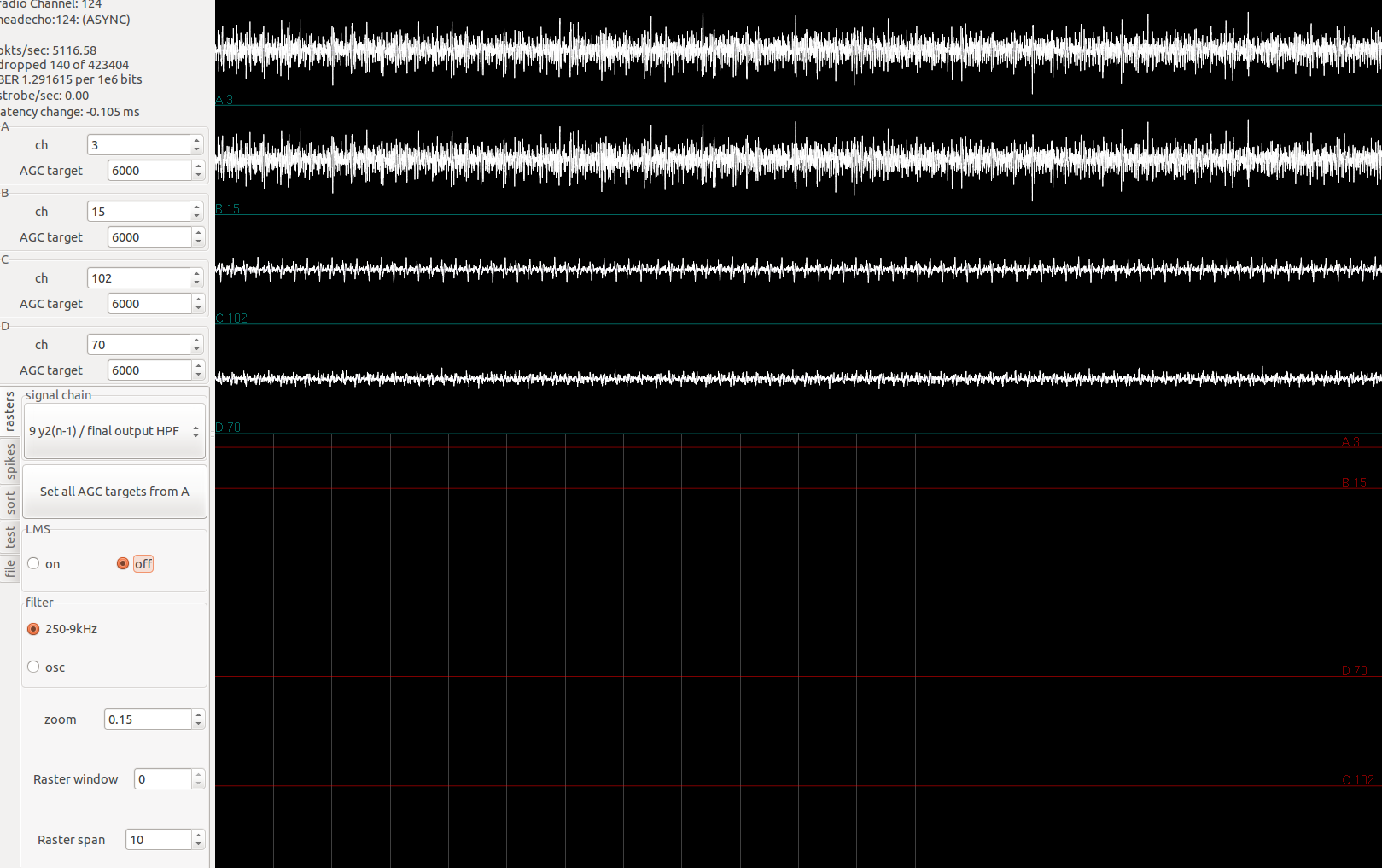
Waveform display
Each received wireless packet has 24 bytes of waveform data nd 8 bytes of template matching data. The waveform data is in fact 6 consecutive samples from 4 different channels, each sample is one byte in size. However, it is important to know how we are supposed to interpret this byte value before plotting.
In my earliest iteration of radio_basic.asm firmware, I am simply saving the high byte of the 16-bit sample acquired from the RHD2132. The amplifiers were configured to transmit the samples in offset-binary, meaning the most negative voltage with respect to the reference electrode is represented by 0x0000, the most positive 0xffff, and the reference voltage is 0x7fff. Therefore, I would want to treat the byte extracted from the packet as an unsigned char. The waveform plot window has vertical range of [-1,1], therefore to plot, I had mapped the unsigned char range [0,255] to [-1,1].
In later firmware iterations, AGC and IIR filter outputs are transmitted. Those samples, however, have to be interpreted as signed char. This is because the samples collected were converted to signed Q1.15 before going through the signal-chain process, and therefore the outputs ended up in signed two’s complement format as well.
Although the location of the decimal point varied depending on what the value transmitted is. For example, the AGC gain is Q7.8, therefore the decimal point is at the end of the most significant byte being transmitted. In comparison, the result of IIR filter is Q1.15, so the decimal point is after the most significant bit of the byte transmitted in that case. But since we are never mixing displaying waveforms in different format, this is not too important, just have to keep in mind when interpreting the waveforms plotted. Although practically speaking, the shape of the waveforms is the most important for spike-sorting, debugging, etc.
In those cases, to plot, I had to map the signed char range [-128,127] to [-1,1], which is a different function from the signed char mapping.
The gtkclient by default used the signed char mapping. Therefore when I first transmitted Intan data as unsigned data, the waveforms plotted were simply rail-to-rail oscillations due to value-wrappings. There are two ways to allow displaying both Intan data and the signal chain data appropriately:
Changed the mapping based on what part of the siganl chain gtkclient has selected from the headstage to transmit.
Configure the RHD2132 to transmit samples in two’s complement format. This actually simplifies the AGC stage. Since the signed 16-bit samples can be treated as Q1.15 numbers right-away, we skip a step of conversion from unsigned to signed fixed-point. With this method, gtkclient can use the signed char mapping to display all parts of the signal chain.
Multicast Problems
This problem happened during a demo of the wheelchair experiment using RHA-headstages, with RHA-gtkclient running on Daedalus. A router was used rather than a switch at a time. Despite router configurations to not filter multicast traffic, the bridges were not able to be detected by gtkclient.
UDP sockets opened by gtkclient:
4340, and 4340+radio_channel are the bcastsock to detect bridges. This is what we are interested in for the bridge problem.
4343: TCP server socket to receive BMI3 connections
8845: Strobe socket
Steps:
Used ss -u -a to check what multicast sockets are open.
Monitor multicast traffic via wireshark:
sudo tshark -n -V -i eth0 igmp
Surprisingly, after executing this command, we started to receive bridge packets and gtkclient started working again.
I wasn’t able to duplicate this scenario on other systems…
While trying to confirm that the radio transmission for the RHD-headstage firmware was working correctly, I needed a way to decouple the signal-chain from the transmission in terms of testing. A nice side-effect of the cascading biquad IIR filter implementation is that, by writing coefficients for the biquads in a certain way, sinusoidal oscillations for different frequencies can be generated. If this was done on the last biquad, it would result in pure sinusoids being transmitted to gtkclient (when the final output is selected for transmission, of course), and it would be easy to see if the data is getting corrupted in the transmission process (if not, then any corruption would be due to the signal-chain code).
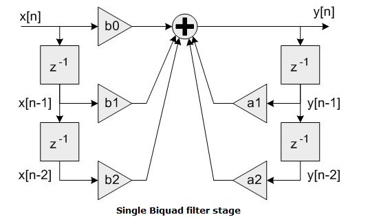
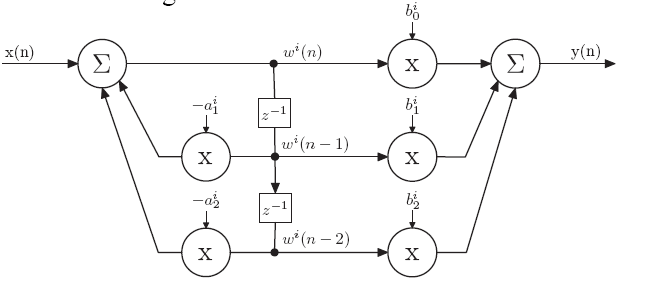
Below is the the DI-biquad block diagram again:
If we assume nonzero initial conditions such that \(y[n-1]\) and \(y[n-2]\) are nonzero, then pure oscillations can be induced by setting \(b_0\), \(b_1\) and \(b_2\) to be 0, in which case only feedback is present in the biquad.
The system function is then:
\[\begin{align}
Y &= a_1z^{-1}Y + a_2z^{-2}Y \\
\end{align}\]
Let \(a_1=2-f_p\), and \(a_2=-1\), then the resulting conjugate poles will be at
The resulting normalized frequency of oscillation is \(\omega=\angle{p_1}\), in radians/sample. Oscillation frequency in Hz is \(f=\frac{\omega F_s}{2\pi}\), where \(F_s\) is the sampling frequency (in our case 31.25kHz for all channels).
So all we need to find is \(fp\) to get a desired oscillation frequency. To find the appropriate coefficients for the last biquad of my signal to induce oscillations, I used the following Matlab script. Note that the coefficients naming is different from that in the diagram – \(a_0\) and \(a_1\) in script are the same as \(a_1\) and \(a_2\) in diagram.
% IIR oscillator - myopen_multi/gktclient_multi/matlab/IIR_oscillator.mFs=31250;% sampling frequency% To get oscillator of frequency f, do:% set b0=0, b1=0, a1=-1, and a0=2-fpfp=0.035;omega=angle((2-fp+sqrt(fp^2-4*fp))/2);% in rad/samplef=omega*Fs/(2*pi);% convert to Hz% But a0 is fixed-point number, convert fp:fp_fixed=round(fp*2^14);% coefficientsb0=0;b1=0;a0=(2^15-fp_fixed)/2^14;a1=-1;y=[0.5,0.5];% y[n-1]=0.5, y[n-2]=0.5x=rand(1,1002)*2;% 1000 random values, including x[n-1] and x[n-2]fori=3:numel(x),val=b0*x(i)+b1*x(i-1)+b0*x(i-2)+a0*y(i-1)+a1*y(i-2);y=[y,val];endplot_fft(y,31250);
The signal chain ends after IIR, at which spike matching happens.
Spike Templates
Spike templates are generated through spike sorting on gtkclient, then transmitted to and saved by the headstage. Spike sorting through PCA is described very well in Tim’s thesis:
Spike sorting on the client is very similar to that used by Plexon Inc’s SortClient and OfflineSorter: raw traces are thresholded, waveforms are extracted around the threshold, and a PCA projection is computed of these waveform snippets. Unlike Plexon, threshold crossing can be moved in both time and voltage domains, which permits considerably greater flexibility when centering a waveform within the relatively narrow 16-sample template region. […] PCA projected waveforms are selected by the user via a polygonal lasso, and the mean and L1 norm of this sample is computed. The former is sent to the transceiver as the template, and the latter sets a guess at the aperture. Aperture can later be updated manually by the user; as the aperture is changed, the GUI updates the color labels of the PCA projected points.
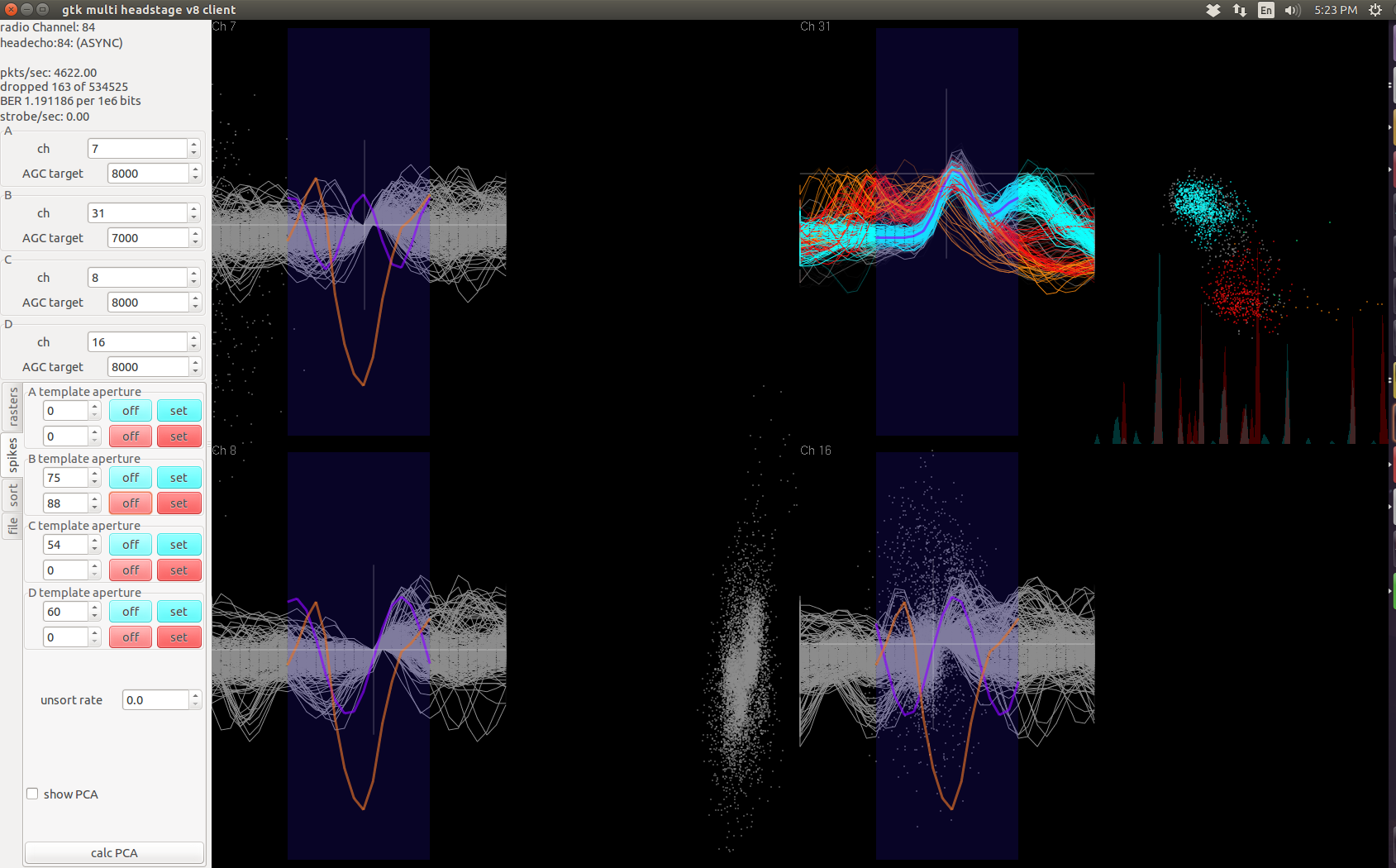
Image below shows spike-sorting in action:
Note that this PCA template process can apply to any signal shape, not just limited to a neural signal waveform. In the screenshot, channel 31 is just noise when projected into the PCA space vaguely forms two clusters. The overlaid waveforms (cyan and red) don’t resemble any neural signal. But the fact that they overlaid simply tells us that the noise detected on channel 31 is not purely stochastic and probably contains interference from deterministic sources.
The 16-point templates in the time domain is limited only to the purple strip in the waveform window. For each channel, a maximum of two set of 16-point templates (16 8-bit numbers) can be stored on the headstage. For each template, the corresponding aperture is also stored as a 8-bit number.
Blackfin Implementation
The assembly implementation of template matching on blackfin (without LMS) is as below:
// At end of signal chain for both group of two samples
// Template comparison, plexon style. Sliding window, no threshold.
// r2=samples from amp1 and amp2; r3=samples from amp3 and amp4. Pack them
r2 = r2 >>> 8 (v); // vector shift 16-bit to 8 bits, preserve sign
r3 = r3 >>> 8 (v);
r4 = bytepack(r2, r3); // amp4,3,2,1 (hi to low byte)
r0 = [FP - FP_8080]; // r0=0x80808080;
r4 = r4 ^ r0; // convert to unsigned offset binary. SAA works on unsigned numbers.
r0 = r4; // save a copy for later
.align 8; // template A: load order is t, t-15, t-14,...t-1
a0 = a1 = 0 || r2 = [i0++]; //r2=template_A(t), r0 and r4 contains byte-packed samples just collected
saa( r1:0, r3:2 ) || r0 = [i3++] || r2 = [i0++]; //r2=template_A(t-15), r0=bytepack(t-15)
saa( r1:0, r3:2 ) || r0 = [i3++] || r2 = [i0++]; //r2=template_A(t-14), r0=bytepack(t-14)
saa( r1:0, r3:2 ) || r0 = [i3++] || r2 = [i0++]; //r2=template_A(t-13), r0=bytepack(t-13)
saa( r1:0, r3:2 ) || r0 = [i3++] || r2 = [i0++]; //r2=template_A(t-12), r0=bytepack(t-12)
saa( r1:0, r3:2 ) || r0 = [i3++] || r2 = [i0++]; //r2=template_A(t-11), r0=bytepack(t-11)
saa( r1:0, r3:2 ) || r0 = [i3++] || r2 = [i0++]; //r2=template_A(t-10), r0=bytepack(t-10)
saa( r1:0, r3:2 ) || r0 = [i3++] || r2 = [i0++]; //r2=template_A(t-9), r0=bytepack(t-9)
saa( r1:0, r3:2 ) || r0 = [i3++] || r2 = [i0++]; //r2=template_A(t-8), r0=bytepack(t-8)
saa( r1:0, r3:2 ) || r0 = [i3++] || r2 = [i0++]; //r2=template_A(t-7), r0=bytepack(t-7)
saa( r1:0, r3:2 ) || r0 = [i3++] || r2 = [i0++]; //r2=template_A(t-6), r0=bytepack(t-6)
saa( r1:0, r3:2 ) || r0 = [i3++] || r2 = [i0++]; //r2=template_A(t-5), r0=bytepack(t-5)
saa( r1:0, r3:2 ) || r0 = [i3++] || r2 = [i0++]; //r2=template_A(t-4), r0=bytepack(t-4)
saa( r1:0, r3:2 ) || r0 = [i3++] || r2 = [i0++]; //r2=template_A(t-3), r0=bytepack(t-3)
saa( r1:0, r3:2 ) || r0 = [i3++] || r2 = [i0++]; //r2=template_A(t-2), r0=bytepack(t-2)
saa( r1:0, r3:2 ) || r0 = [i3++] || r2 = [i0++]; //r2=template_A(t-2), r0=bytepack(t-1)
saa( r1:0, r3:2 ) || [i3++] = r4; // write bytepack(t), inc i3
// saa results in a0.l, a0.h, a1.l, a1.h (amp4,3,2,1); compare to aperture
// i0 @ Aperture[amp1A, amp2A]
r0 = a0, r1 = a1 (fu) || r2 = [i0++] || i3 -= m3; // r2=aperture[amp1A,amp2A], i3@saved bytepack(t-15)
// subtract and saturate - if the answer is negative-->spike!
r0 = r0 -|- r2 (s) || r3 = [i0++]; // r0=[amp1A match, amp2A match], r3=aperture[amp3A,amp4A]
r1 = r1 -|- r3 (s); // r1=[amp3A match, amp4A match]
// shift to bit 0, sign preserved
r0 = r0 >>> 15 (v); // r0.h and r0.l will be 0xffff or 0x0000 (match or not)
r1 = r1 >>> 15 (v);
r0 = -r0 (v); // now 0x0001 or 0x0000 (match or not)
r1 = -r1 (v); // save both for packing later
r1 << = 1;
r6 = r0 + r1; // r6=[14 zeros][amp4A][amp2A][14 zeros][amp3A][amp1A]
In non-LMS versions of firmware, incrementing by m3 moves address up by 16 32-bit words. In LMS-verions of firmware, incrementing by m3 moves address up by 2 32-bit words.
As mentioned in the Blackfins-Intan post, Blackfin works efficiently with two 16-bit samples at once, therefore the signal-chain operates twice before reaching the template matching step, once for each two samples acquired in a SPORT cycle.
This efficiency is due to Blackfin’s dual-MAC architecture, which can also operate on 4 unsigned 8-bit samples at the same time (treating each byte as a separate number).
Template matching implemented here is simply subtracting the 16 template points from a channel’s current and 15 past samples, then comparing the sum of their absolute differences to the aperture value. If the sum is smaller, then we declare a spike has been detected.
Luckily, Blackfin has the SAA instruction, which accumulates four different sums of absolute difference between vectors of unsigned bytes. Therefore, at the end of the signal chain after all four samples acquired have been processed, they are packed into a 32-bit word by first converting each signed 16-bit sample to offset binary, then take the most significant byte (line 1-7). These bytepacked words are saved for the past 15 samples for each group of four channels in a circular buffer.
The template vectors from the headstage are also written into memory in the same bytepacked form. Thus template matching becomes 16 successive SAA instructions (line 11-27).
Line 31-38 does the comparison between the SAA result against the saved template, resulting in either 0 for no match, or 1 for a match.
Consequences of this method
This biggest upside of this spike matching method is its speed and simplicity of implementation. However, despite the simplicity, this is probably not the most optimal or correct method for spike detection because:
In most sorting algorithms (e.g. Plexon), the raw signal is first thresholded, then waveform snippets of usually 32 samples long are compared to a template to accept/reject, or to sort them into different units. The comparison metric, or aperture in our implementation, is usually the MSE or L2-norm. Our implementation uses 16-sample window and L1-norm, which presumably may have worse performance.
Because the spike-sorting is based on 16-bit samples truncated to 8-bit samples, the templates themselves have truncation noise. The onboard spike-matching also involves truncation of the samples. How this truncation noise can affect the sorting quality has not been rigorously studied. But I expect this to not contribute significantly to spike-detection performance hit (if at all).
Literature suggests that for isolating a fixed-pattern signal embedded in noise, the best solution might be matched filter, which Tim has done a preliminary study on.
L1 data memory - consists of 2 banks of 2-way associative cache SRAM, each one is 16kB.
databank A: 0xFF804000 to 0xFF808000
databank B: 0xFF904000 to 0xFF908000
L1 scratchpad RAM - accessible as data SRAM, cannot be configured as cache memory, 4kB. Address is (0xFFB00000 to 0xFFB010000)
For our firmware, we want to load:
The instructions into the 32kB SRAM instruction memory.
Signal chain calculations and intermediate values (W1), past samples for template comparison (T1), template match bits (MATCH) , look-up tables (ENC_LUT and STATE_LUT), and radio packet frames to L1 databank A.
Signal chain coefficients/parameters (A1), template and aperture coefficients (A1), and pointer values (FP_) to L1 databank B.
These memory layout and address are visualized in each firmware directory’s memory_firmwareVersion.ods files, and memory_firmwareVersion.h header files.
To compile our code to fit this memory structure, we use the blackfin linux bare-metal tool chain, which is a gnu gcc based toolchain that allows us to compile assembly and c/c++ code for different blackfin architectures. The installation comes with header files such as defBF532.h that lists the memory addresses for various MMRs and system registers.
After running make, the file Linker.map shows the order of files linked in the final stage.dxe file, which includes:
crt0.o - from crt0.asm. Includes the global start() routine from where BF532 starts execution. Also includes most of the processor peripheral setup, such as PLL and clock frequency, and interrupt handler setup.
radio_AGC_IIR_SAA.o - from radio_AGC_IIR_SAA.asm, this is where awherewherewhere all the DSP and interesting code go. The different firmware versions only really differ in this file.
enc.o - generated by enc.asm, generated by enc_create.cpp. It’s a subroutine called in the data memory setup code in radio_AGC_IIR_SAA.asm to install the encoding look-up tables.
divsi3.o - generated by common_bfin/divsi3.asm, a subroutine for signed division…not really actually used, but could be useful.
main.o - from main.c. The blackfin starts execution from crt0.asm, which eventuall jumps to the main routine within main.c. Within the main routine, more blackfin and Nordic radio chip configurations are done. The radio setup is done throught the SPI interface (such as the radio channel). At the end of main(), it jumps to the setup-up code radio_bidi_asm within radio_AGC_IIR_SAA.asm.
print.o - from common_bfin/print.h and common_bfin/print.c. Not actually needed for the headstage, rather a leftover from compilation setup for BF537. Not really relevant to headstage firmware.
util.o - from common_bfin/util.h and common_bfin/util.c. Functions defined not actually needed for the headstage.
spi.o - from common_bfin/spi.h and common_bfin/spi.c. Include functions in C to talk to the SPI port, which is needed for reading the flash memory and talking to the radio - functions called from the main() routine.
Finally, the file bftiny.x is the linker script to produce the final binary .dxe file. Written by unknown author, but it works!
The assembly version of the final compiled code and their memory addresses can be found in decompile.asm. The code order follows the link order. See this document for more details on the compile process.
The flash process will upload the final stage.dxe file into the onboard flash memory. The blackfin is wired to boot from flash - upon power up, blackfin will read the flash memory through SPI and load the data and instructions to the corresponding memory addresses appropriately.
The architecture of the firmware (in radio_AGC_IIR_SAA.asm for RHD-headstage or radio5.asm for RHA-headstage) is essentially two threads: DSP service routine reads in samples from the amplifiers and does the DSP, the radio control thread handles radio transmission and reception.
The radio control thread (radio_loop) fills the SPI read/write registers and changes flags to the radio to transmit packets. It also reads the incoming packets and writes the desired changes to the requested memory locations. Interleaved between these instructions, the DSP service routine is called.
The DSP service routine blocks until it receives until a new set of samples (4 samples, one from each amplifier) is read and fully processed and then returns control back to the radio control thread. To preserve state for each routine, circular buffers are used to store:
DSP signal-chain constants and coefficient values (A1).
Past stored samples for spike detection (T1).
Data to be transmitted by the radio (packet buffer).
After all amplifier channels have been processed once, template matches and raw samples are written to the packet buffers. The radio-control thread monitors the packet buffer and transmit when packets are available.
One key limit to this threading architecture is the ADC sampling rate. The processor is operating at 400MHz. The ADC onboard the Intan operates at 1MHz. That means the code-length for calling the DSP service routine, return and execute an instruction in the radio loop, then back, cannot exceed 400 clock cycles.
Whenever the code-length violates this limit, data corruption and glitches can happen.
Outside of the values stored in the circular buffers, all persisten variables that do not have their own registers, such as the number of packets enqueued, are stored in fixed offsets from the frame pointer to permit one-cycle access latency.
The memory map spreadsheet is very helpful in debugging and understanding code execution.
The radio-transmission protocol is described fairly well in Tim’s thesis pg. 166-168.
Some important points to remmember and references:
Each 32-bytes radio packet contains, in order of low to high byte:
6 samples from 4 channels of raw data (on any part of the signal chain selected by gtkclient).
8 bytes of template matching.
Each byte indicates whether there is a spike detected for both templates of a group of 4 channels - if each bit represents one template on one channel, then all 8 bits of the byte will be taken. However, we make the assumption that the two neurons represented by the two templates on the same channel cannot both fire at the same time, this then allows an encoding scheme to compress the matching byte into only 7bits. The most-significant bit in the first four template-matching bytes are then replaced by the bits of an packet # in frame nibble. This nibble ranges from 0-15, representing the position of the current packet within the 16-packets radio frame.
The next four template-matching bytes has their most significant bit replaced by the bits of an echo nibble. This echo nibble is extracted from the last command packet gtkclient sent to the headstage, and allows a sort of SEQ-ACK exchange to happen between the headstage and gtkclient, although this only allows to know when a packet might’ve been lost – there is no bandwidth or CPU cycles to resend a lost packet. However, the control packets can be resent easily. The Sync headstage in gtkclient is a good way of sending control packets to sync the headstage configurations to those in gtkclient.
There are a total of \(32 \frac{channels}{amplifier} \times 4 \frac{amps}{headstage} \times 2 \frac{matches}{channel}=256 \frac{matches}{headstage}\), meaning it takes 4 packets to transmit all template matches, accompanied by 24 samples of 4 channels.
ADC runs at 1Msps, each packet requires 6 samples, so each packet requires \(\frac{6 samples\times 32 channels/sample}{1Msps}=192\mu s\), and 4 packets requires \(768\mu s\) to transmit.
Firmware sets aside a buffer enough for two radio frames. Each radio frame contains 16 packets. The radio starts sending when a frame is full, while the signal-chain collates and saves new packet in the other frame. Therefore, each frame takes about 3.072 ms to send, which is less than the 4ms free-run PLL time. Time to transmit, change to receive, then back is 3.60ms. So,
Received packet are 4 (memory address, value) pairs. Each value is 32 bits. Memory address should be 32bits, but since their upper nibble is always 0xf, they are replaced with the 4 bits echo value. In the radio loop handling received packets, the echo value is extracted and saved, while the memory address is restored. The values from the packets are then written to the corresponding memory address.
Debugging Notes
If the firmware used on headstage allows for radio transmission (i.e. radio_loop implements the described protocol), there are several ways to debug and check the quality of transmission.
If the headstage’s firmware is compiled correctly, the bridge’s firmware is compiled correctly, gtkclient is compiled correctly, and multicast is allowed, yet there are not signals showing up in gtkclient, then there is something wrong with the radio code within the headstage’s firmware.
If the gtkclient is getting raw waveforms displayed, but the waveforms look suspicious: for example, we apply sinusoids signals but waveforms displayed aren’t very smooth, that may be caused by either errors in DSP or radio transmission code. We can eliminate the former possibility if after gtkclient instructs the headstage to change coefficients to induce oscillations (see IIR oscillator post) we do indeed see sinusoids of the same frequency on all transmitted channels.
In gtkclient, if the pkts/sec field is changing, but the dropped and BER fields stays constantly 0, that means something is wrong with the radio packaging process. As great as 0 dropped packet sounds, it very unlikely.
I encountered these last two problems while finalizing the RHD-headstage firmware.
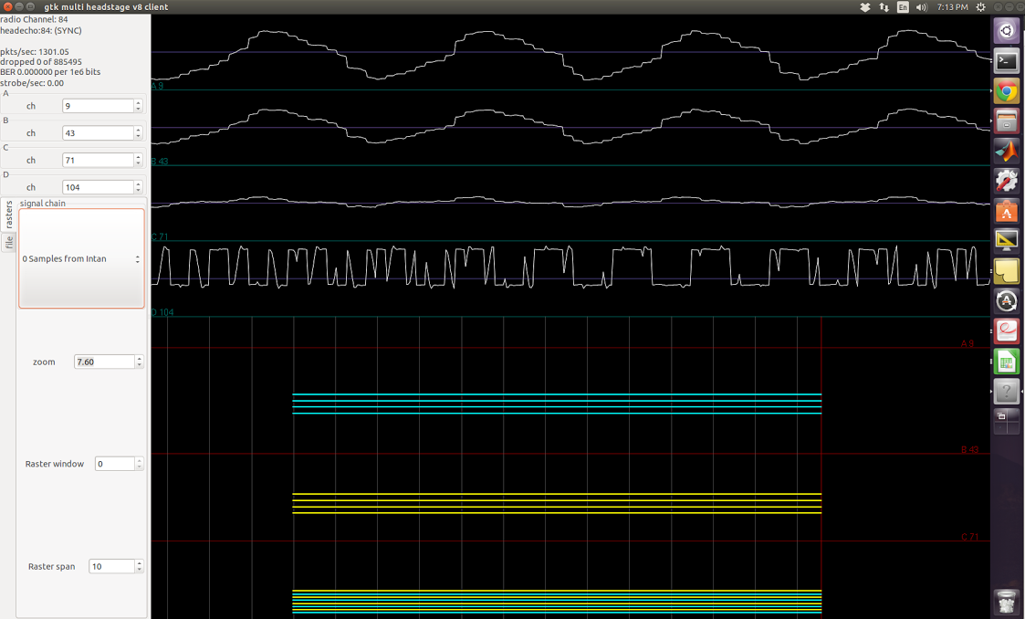
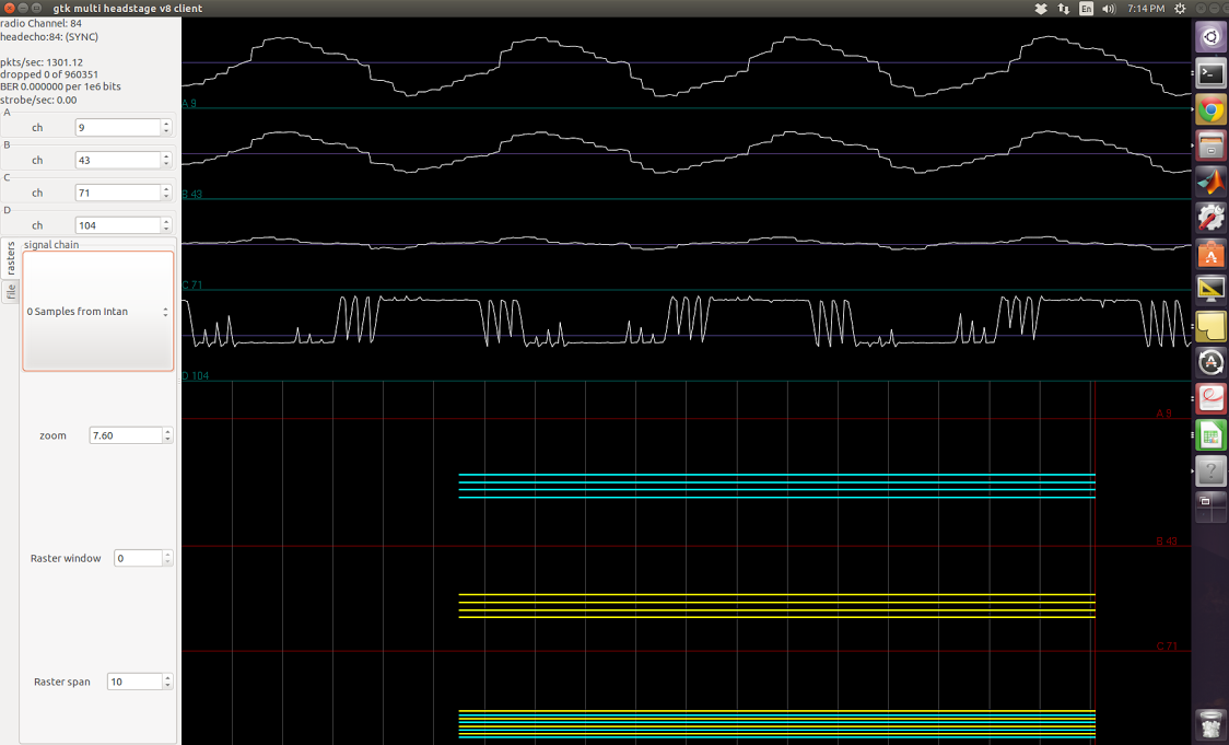
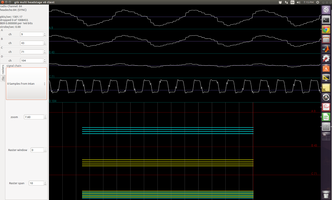
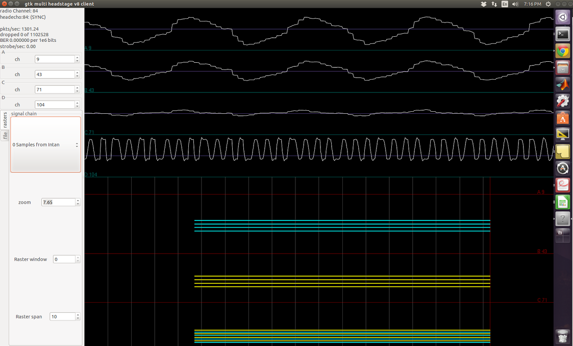
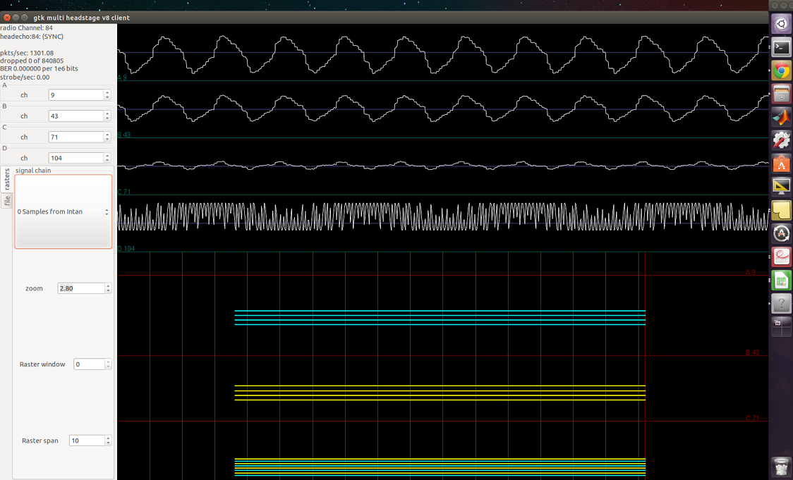
In the screenshots below, I applied square waves of known frequency to one of the amplifiers. The top three channels are floating, the fourth one is supposed to be the sinusoid applied. The firmware I used does not have any signal-chain steps so I was simply streaming the acquiared samples from Intan.
800Hz signal applied
1kHz signal applied
1.2kHz signal applied
1.5kHz signal applied
2kHz signal applied
2.8kHz signal applied
It is apparent in most of these screenshots that I’m not getting a square wave back. In others, I get resemblance of square wave, but the frequency is never right, and the waveform seems to have multiple frequencies present, both higher and lower than what I expect.
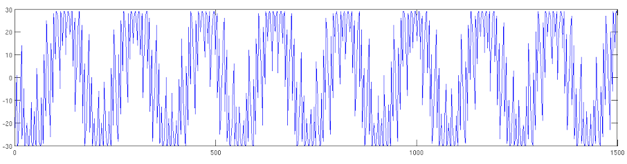
Transmitting the IIR-generated oscillations also showed distortions. The generated waveform is supposed to be 919Hz. The recorded signals, when dumped and plotted in Matabl is shown below:
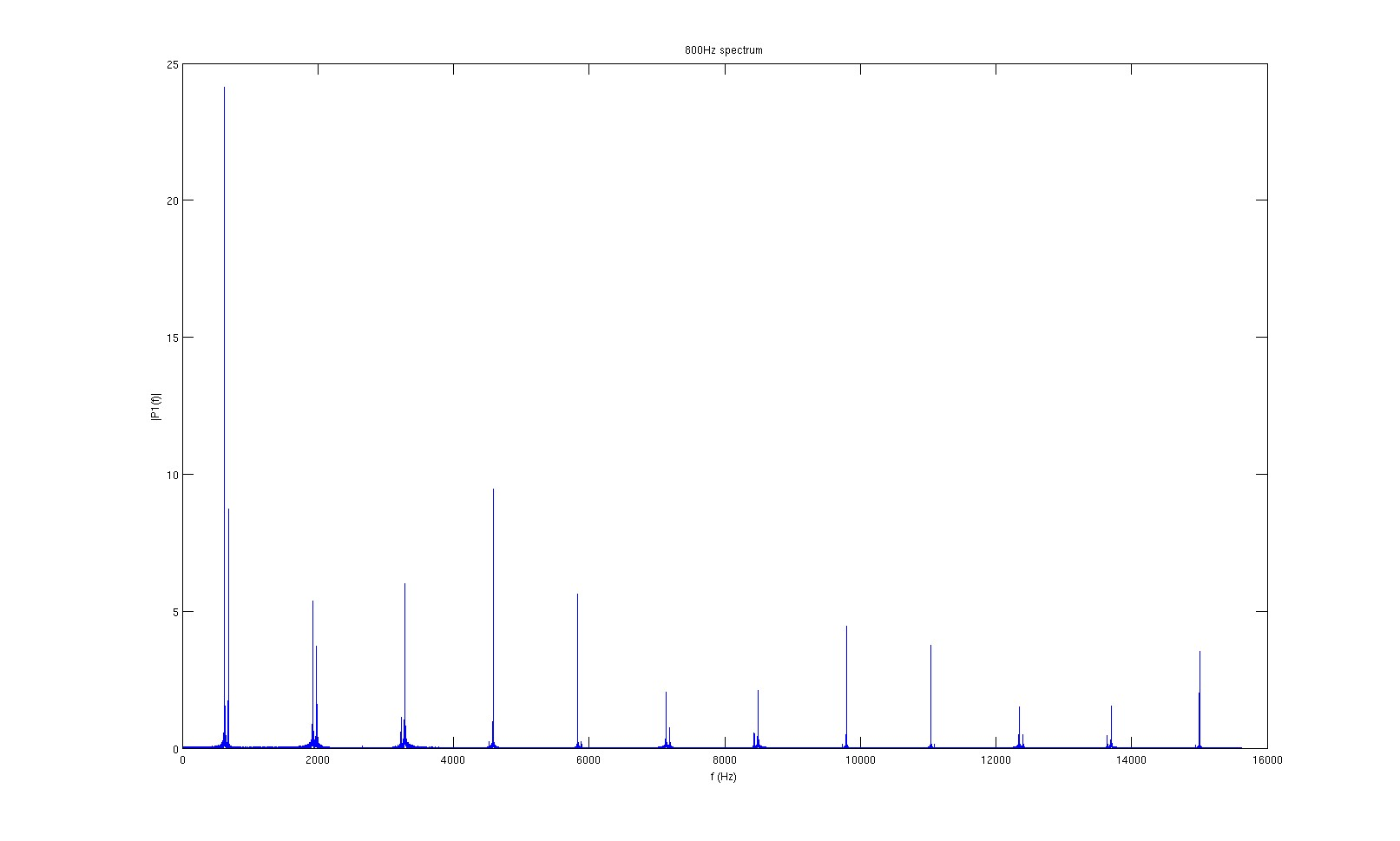
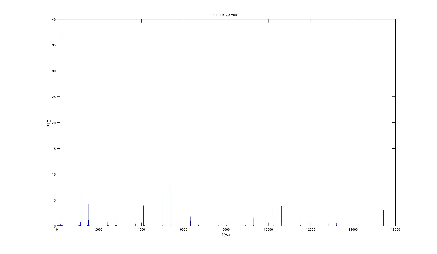
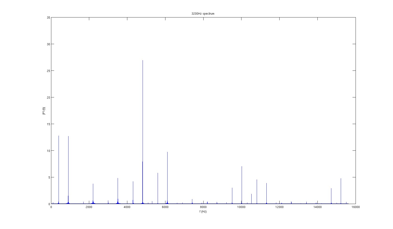
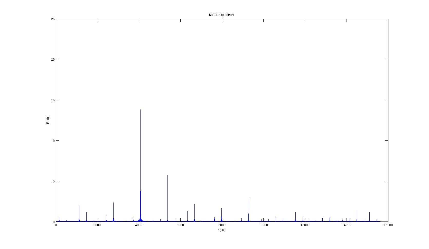
The first idea that came to mind to investigate what’s going on was performing FFT. Below are FFT of gtkclient recording when sinusoidal signals of different frequency was applied, as well as that of the IIR-generated oscillations.
800Hz signal FFT
1kHz signal FFT
3.2kHz signal FFT
5kHz signal FFT
None of the spectra look very clean, and the signal’s actual frequency never has the most energy. However, it seemed that the highest peaks are consistently 1300Hz apart. Since the sampling frequency of the amplifiers is 31.25kHz, 1300Hz correspond to every 24 samples, or every 4 packets.
In the radio-transmission protocol, the spike-match bits are looped every 4 packets – the spike match bits rae saved in a buffer, and for every packet a pointer reads through this buffer. The pointer loops should therefore loop around the buffer every 4 packets, since all spike-match bits are transfered in that time.
Very careful line-by-line inspection of the radio packet assembly/transmission code revealed that I made a mistake modifying the original transmission code when modifying to work with firmware versions that did not include SAA template-matching. Fixing those errors solved the problem in all non-final RHD firmware versions.
That would mean after adding SAA, I only needed to copy over the original radio packet assembly/transmission code from RHA-headstage’s radio5.asm to get everything work. But it didn’t, and the same 1300Hz problem appeared. This then led me to a typo in my initial memory-allocation code in radio_bidi_asm, executed even before any of the signal-chain or radio-loop threads.
More Resources
Tim has notes on his radio protocol hardware/software development on his website, good read in case of any future Nordic radio work.
LMS is the second stage of processing in RHA-headstage’s signal chain, after AGC. It aims to estimate the noise common to all electrodes and subtract that noise from each channel.
Adaptive Filtering Theory
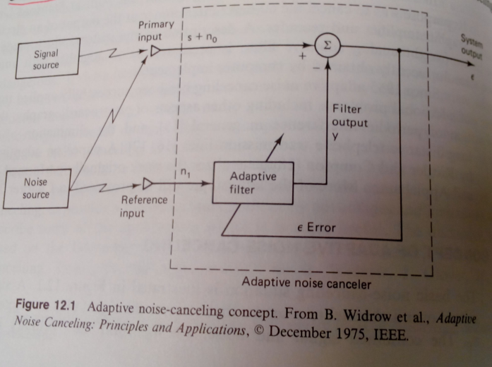
Chapter 12 on Adaptive Interference Cancelling in Adaptive Signal Processing by Bernard Widrow is an excellent reference on adaptive interference cancelling. Chapter 6 is a great reference on the LMS algorithm.
In adapative noise cancelling, we assume the noise source injects into both the primary input and the reference input. THe signal of interest is localized in the primary input. An adaptive filter then tries to reconstruct the noise injected by combining the reference inputs. This approximation (\(y\) in the figure below) is subtracted from the primary input to give the filtered signal (\(\epsilon\)). This filtered output \(\epsilon\) is then fed back into the adaptive filter to tune the filter weights. The rationale is that the perfect adaptive filter will perfectly approximate the noise component \(n_0\), \(\epsilon\) will then become \(s\), and the error signal is minimized.
An interesting question is, why would \(\epsilon\) not be minimized toward 0? If we assume the signal \(s\) is uncorrelated with the noise \(n_0\) and \(n_1\), but \(n_0\) and \(n_1\) are correlated with each other, then the minimum \(\epsilon\) can achieve, in the least mean squared sense, is equal to \(s\). Unfortunately, this results is less intuitive and more easily seen through math (Widrow and Bernard, Ch 12.1).
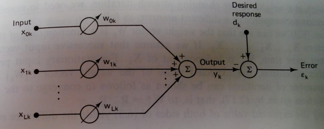
Another way of seeing LMS filtering is that, in LMS, given an input vector \(\vec{x}\), we multiply it by weights vector \(\vec{w}\) such that we reduce the least-mean-squared error, which is the difference between \(w^T x\) and the desired vector \(\vec{d}\). The error term is then fedback to adjust \(\vec{w}\). This is illustrated below:
In the case of adaptive filtering, the desired response \(d_k\) is the noise component present in the primary input (\(n_0\)). In fact, for stationary stochastic inputs, the steady-state performance of slowly adapting adaptive filters closely approximates that of fixed Wiener filters.
A side tangent is, why dont we use LMS with Wiener filter in BMI decoding? In this case, the adaptive filter output \(y\) and \(\epsilon\) would have to be decoded covariates, it is difficult to see how that would increase decoding performance.
In contrast with Wiener filter’s derivation where we estimate the gradient of the error in order to find \(\vec{w}\) values to minimize the error, in LMS, we simply aprroximate the gradient with \(\epsilon_k\). This turns out to be an unbiased estimator, and the weights can be updated as:
where \(\mu\) is the update rate, similar to that in other gradient descent algorithms.
Therefore, the LMS algorithm is a rather simple algorithm to serve as the adaptive filter block in the adaptive noise cancellation framework.
Application in firmware
To apply these algorithms to our headstage application, we treat the current channel’s signal as \(s_n+e_n\), where \(s_n\) is the signal for channel \(n\), \(e_n\) is the noise added to channel \(n\) at current time \(t\). \(e_n\) can be assumed to be Gaussian (even though in reality it probably isn’t, e.g. chewing artifacts). It’s reasonable to assume that \(e_n\) is correlated with noise observed in other channels (since they share the same chip, board, etc): \(e_{n-1}\), \(e_{n-2}\), etc. The signals measured in the previous channels then can be used as the reference input sources to predict and model the current channel’s noise.
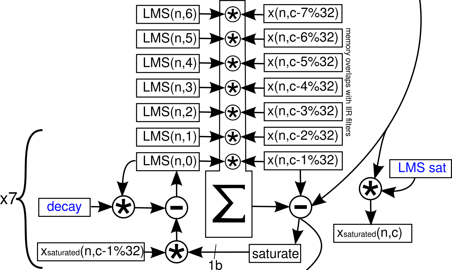
This is implemented in the firmware by Tim Hanson as below:
This is described by Tim in the following diagram, where \(c\)=current channel number, \(n\)=current sample number.
Prior to start of line 12, i1 points to AGC gain of current channel \(c\), i2 points to the integrator mean of current channel, i0 points to AGC transfer function coefficients prior to LMS coefficients.
Line 12: r3 will contain the updated AGC gain, and r7 will contain the weight decay for LMS. The weight decay will be either 0 or 1 in Q15. 0 effectively disables LMS.
Line 13: r0 currently contains AGC output. The multiplication will multiply the AGC output by weight decay, saturate the sample and move it to r4. Updated AGC gain from the previous step is saved by writing to i2, which is then incremented to point at saturated AGC output. i1 is moved to point to the AGC gain value corresponding to channel \((c-7)\%32\).
Line 17: The saturated sample of channel \((n-7)\%32\) is loaded into r1, i1 now points to AGC output for channel \((c-7)\%32\). The current channel’s saturated AGC sample in r4 is saved, and i2 now points to current channel’s AGC-output (from sample n-1).
Line 18: r1 is loaded with AGC output of channel \((c-7)\%32\). i1 points to AGC output of channel \((c-6)\%32\). r2 is loaded with the LMS weight corresponding to channel \((c-7)\%32\), or \(LMS(n,6)\) in diagram.
Line 19: a0 contains the product of \(LMS(n,6)*x(n,c-7\%32)\) in figure above. r1 is loaded with AGC output of channel \((c-6)\%32\) while i1 end up pointing to AGC output of \((c-5)\%32\). r2 is loaded with \(LMS(n,5)\) while i0 end up pointing to \(LMS(n,4)\).
Line 20-24: Continues the adaptive filter operation (the multiply/summation block in diagram). At end of line 24, r1 contains AGC output of \((c-1)\%32\), i1 is moved to point to AGC out of \(c\). r2 is loaded with \(LMS(n,0)\), i0 is moved to point to low-pass filter coefficients.
Line 25: r6 now contains the result of the entire multiply-accumulate operation of the linear combiner (\(y_k\) in figure 2). r1 is loaded with AGC out of current channel, i1 is then moved to point at AGC out of \((c-7)\%32\). r2 is loaded with low-pass filter coefficients and moved back to point to \(LMS(n,6)\). The r1 and r2 values will not be used and will be overwritten next instruction.
Line 28: r0 originally contains current channel’s AGC output. Subtracting r6 from it, r0 will contain the LMS filtered output – \(\epsilon=s+n_0-y\) in figure 1. Meanwhile, the current AGC output is written, after which i2 will point to the delayed sample used for IIR filters. r1 is loaded with AGC out of \((c-7)\), after which i1 points to saturated AGC output of \((c-7)\%32\).
Line 29: After shifting r0 vectorially, r6 is loaded with the sign of filtered LMS output, or \(sign(\epsilon)\). r1 is loaded with saturated AGC output of \((c-7)\%32\), i1 then points to saturated AGC output of \((c-6)\%32\). r2 is loaded with the corresponding LMS weight \(LMS(n,6)\), i0 then points to \(LMS(n,5)\).
Line 33-34: Update the weight \(LMS(n,6)\). r5 will contain the updated weight equal to \(w*\alpha+x*sign(\epsilon)\), where \(w\) is the LMS weight, \(\alpha\) is either 0 or 1 indicating whether LMS is on, \(x\) is the saturated AGC output corresponding to the weight, and \(\epsilon\) corresponds to current channel’s filtered LMS output.
End of line 34, r1 is loaded with saturated AGC output of \((c-6)\%32\), then i1 points to saturated AGC output of \((c-5)\%32\). r2 is loaded with \(LMS(n,5)\), but i0 points to \(LMS(n,6)\).
Line 35: Here the updated \(LMS(n,6)\) weight is written (hence i0 pointing to that location after line 34), after which i0 skips to point at \(LMS(n,4)\).
Line 36: r5 contains the updated weight \(LMS(n,5)\). r1 is loaded with saturated AGC output of \((c-5)\%32\), i1 points to saturated AGC output of \((c-4)\%32\). r2 is loaded with \(LMS(n-4)\), i0 then points to \(LMS(n,5)\) in anticipation of its update.
Line 46: r5 now contains the last updated weight \(LMS(n,0)\). r1 is loaded with current channel’s saturated AGC-output, then i1 is moved to point current channel’s delayed sample (in anticipation of IIR filter). i0 points to \(LMS(n,0)\).
Line 47: The updated \(LMS(n,0)\) is written back to memory.
The implemented algorithm is a modified LMS approach, where the filter weights are updated by
\(\begin{align}
\vec{W_{k+1}} &= \vec{W_k} + \vec{X_k}*sign(\epsilon_k) \\
&= r2*r7 + r1*r6
\end{align}\)
where the registers are those used in line 33-46.
Here, the old \(w_k\) are loaded into r2. r7 contains a weight-decay factor. If it’s set to 0, LMS is effectively disabled as no weight update would happen and it becomes a fixed gain stage.
r1 contains the saturated version of each reference channel’s input. r6 is the sign of the error term.
In this modified LMS approach, if both the error and sample are the same sign, the weight would increase (Hebb’s rule). This implementation involves saturation and 1-bit weight updates, so it’s not analytical. However, it is fast and according to Tim,
in practice the filter settles to final weight values within 4s. The filter offers 40dB of noise rejection.
If at any time the error term \(\epsilon_k=0\), that means the current channel can be completely predicted by the previous 7 channels, that means the current channel is measuring only noise. This could serve as a good debugging tool.
Finally, at the end of this code block, r0 contains the LMS filtered sample, also \(\epsilon\). The IIR stage following LMS then operates directly on this filtered sample. Therefore only the regular and saturated AGC outputs are saved, while the LMS filter output is not saved until the IIR stage as a delayed sample (after AGC-out slot).
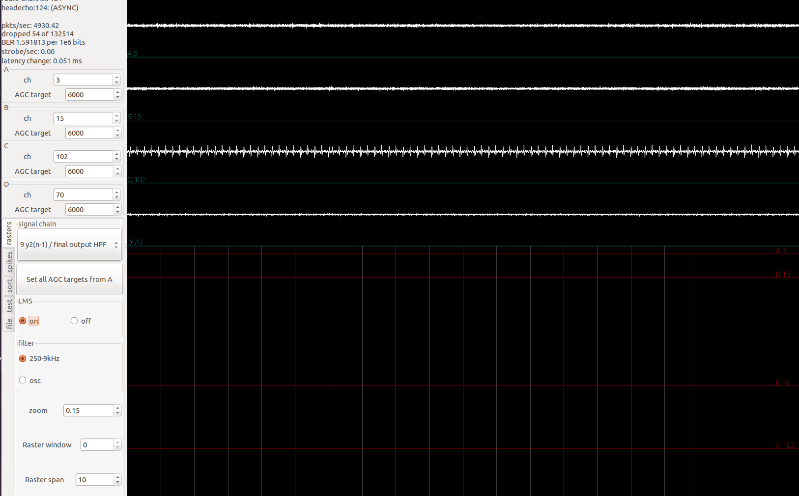
The effects of LMS is especially clear when all the channels of an amplifier is applied the same signal:
Simulated spike signals are being applied through the Plexon headstage tester to channel 0-31. In image shown, the first two channels have fairly low signal. This is expected since all channels have the same signal, the previous 7 channels can exactly reconstruct the signal in the current channel, subtraction leaves little left.
Turning off LMS, we have the following:
The identical spike signals applied now show up loud and clear in the first two channels shown.
This helps a lot. Finally got the syntax higlighting and line numbers to work.
Update: 2/1/2016
Apparently jekyll (written in ruby)’s default highlighter has changed to rouge, because pygments was written in Python and they think it’s too slow to use a ruby wrapper for it.
This means github pages is also using rouge as the default highlighter, which unfortunately does not support assembly. So now all my assembly code snippets are just gray..and the code table is broken, now there is an extra gray box around the actual code box. Too much webdev, maybe fix later.
Continuing to add on to the RHD headstage’s signal chain, I have to cut down on the number of biquads used to implement the butterworth bandpass filters on the Blackfin. The original code uses four back-to-back biquads to implement 8-pole butterworth filter.
The reason for using butterworth filter is because of the maximal flat passband. The reason for using back-to-back biquads rather than a big-chain (i.e. naively implementing the transfer function) is because each biquad uses only one summer, maximizing efficiency on embedded systems.
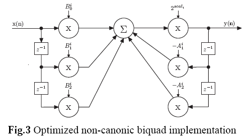
DF2-biquad
DF1-biquad
Most commonly, Direct Form II biquads are used in implementations because only 1 delay line is needed. However, as this great paper and [other common DSP resources] (https://www.amazon.com/Understanding-Digital-Signal-Processing-3rd/dp/0137027419) suggest, Direct Form II biquads have limitations on the coefficient range. Therefore, Direct Form I biquads are more desirable in 16-bit fixed-point applications for its better resistance to coefficient quantization and stability.
A lot of the original implementation rationale of the filters have been discussed in Tim’s post from a long time ago, it was decided that the filters would implement Butterworth type due to the excellent in-band performance. This post will mostly talk about how to generate the coefficients for the filters given the following assembly code structure per this paper again:
This code is the most efficient implementation of DF1-biquad on Blackfin. To implement new filters, we need to
Get new filter transfer function.
Factor the transfer function into biquad forms.
Make biquad coefficients into correct fixed-point format.
Note that since we are only implementing filters that are cascades of biquads, that means any filters that we implement must contain an even number of poles.
There are two approaches for step 1 and 2. Approach 1 is easier for making filters low number of poles. Approach 2 is easier for high number of poles.
Approach 1
Since I only have enough code-path to implement two biquads (instead of four as Tim did), I need one LPF biquad and one HPF biquad. The filter can be designed by:
fs=31250;% sampling frequency% 2nd order butterworth LPF, cutoff at 9kHzfc_LPF=9000;wn_LPF=(fc_LPF/fs)*2;% normalized cutoff frequency (units=pi rad/sample)[b_LPF,a_LPF]=butter(2,wn_LPF,'low');% descending powers of z, const firstA% b_LPF = [0.3665, 0.7329, 0.3665]% a_LPF = [1, 0.2804, 0.1855]% 2nd order butterworth HPF, cutoff at 500Hzfc_HPF=500;wn_HPF=(fc_HPF/fs)*2;[b_HPF,a_HPF]=butter(2,wn_HPF,'high');% b_HPF = [0.9314, -1.8628, 0.9314]% a_HPF = [1, -1.8580, 0.8675]% plot freq-response of bandpass filterfvtool(conv(b_LPF,b_HPF),conv(a_LPF,a_HPF));
The transfer function of a biquad is \(H(z)=\frac{Y}{X}=\frac{b_0+b_1z^{-1}+b_0z^{-2}}{1-a_0z^{-1}-a_1z^{-2}}\). However, the coefficients generated by the butter() function follows the form \(H(z)=\frac{Y}{X}=\frac{b(1)+b(2)z^{-1}+b(3)z^{-2}}{a(1)+a(2)z^{-1}+a(3)z^{-2}}\), so we need to reverse the sign of the last two values in a_LPF and b_LPF.
To make the generated coefficients into the actual values used on Blackfin, we need to be mindful of how many bits they should be. Since the result of the biquad (line 6 from the assembly snippet) uses the (s2rnd) flag, the result of the summer must be Q1.14 (so s2rnd result is Q1.15). This means all coefficients must be within Q1.14 (and hopefully can be represented as such):
1
2
3
4
5
6
7
b_LPF_DSP=round(b_LPF*2^14);% result is [b0,b1,b0]a_LPF_DSP=round(a_LPF*2^14)*-1;% result is [dont-care, a0, a1]% b0=6004, b1=12008, a0=-4594, a1=-3039b_HPF_DSP=round(b_HPF*2^14);a_HPF_DSP=round(a_HPF*2^14)*-1;% b0=15260, b1=-30519, a0=30442, a1=-14213
These resulting coefficients are what I ended up using in the firmware. The two code snippet above is in gtkclient_multi/genIIRfilters.m.
By multiplying the b-coefficients of the low-pass filter, we can increase the DC-gain without changing the shape of the gain curve (equivalent of increasing the in-band gain due to flatness of Butterworth). However, the resulting coefficients must be clamped within [-32768, 32767] so they can be properly stored within 16-bits.
This is desirable if the presence of high frequency noise makes the incoming signal envelope high and limits the gain, then LMS subtract this common noise. With the extra IIR-stage gain, we can amplify the signal in the passband more. It is not applicable to my version of headstage, because the raw samples are alreayd 16-bits. This is now implemented in gtkclient for all firmware versions with an IIR stage.
The total gain of each biquad is limited to the coefficient range in Q15. For LPF, the DC gain can be calculated as the sum of the filter’s feedforward coefficients divided by 1 minus the sum of the filter’s feedback coefficients (in decimal). Keeping the feedback coefficients, multiplying both feedforward coefficients by the same amount increases the DC gain of the LPF biquad by the same. In gtkclient code, we assumed static gain is 1, i.e. 1 minus the sum of the feedback coefficients is equal to the sum of feedforward coefficients. This is not entirely true, therefore, the IIR gain value represents how much extra gain the filter stage would provide over the base gain.
As the feedforward coefficient values have different magnitude, the same gain may saturate just one of the coefficients. In this case the gain scaling may change the filter’s shape. Therefore, in practice, the IIR gain entered should not be greater than [-2.5, 2.5]. To find the max IIR gain possible without saturating, find the smallest feedforward coefficient for the LPF biquad (m_lowpass_coeffs[0,1,4,5] for RHA or m_low_pass_coeffs[0,1] for RHD, in headstage.h, and divide 2 by that number).
Approach 2
The above approach is fine when we need one LPF biquad and one HPF biquad. But say we need an 8th-order buttworht bandpass filter, using the above approach we would need two HPF biquads and two LPF biquads. We can’t simply use two of the same HPF biquads and two of the same LPF biquads. The resulting bandpass filter will have less bandwidth between the -3dB points (two poles at same frequency means sharper roll-off from that point on).
The solution then, requires us to factor the generated transfer function (gtkclient_multi/genIIRfilters2.m):
% design butterworth filter, and derive coefficients for% the cascade of two direct-form I biquadsfs=31250;% 8th order butterworth bandpass filter% B and A in descending order of z[B,A]=butter(4,[1000,9000]/(fs/2),'bandpass');% Factor the numerator and denominator.% First get the roots of num and den: for rootsrB=roots(B);rA=roots(A);% get the polynomials for each biquad, each from two (conjugate) roots% abs to take care of round-off errors - product of conjugate roots cannot be imaginary.pB1=abs(poly(rB(1:2)));% numpA1=abs(poly(rA(1:2)));% denpB2=abs(poly(rB(3:4)));pA2=abs(poly(rA(3:4)));pB3=abs(poly(rB(5:6)));pA3=abs(poly(rA(5:6)));pB4=abs(poly(rB(7:8)));pA4=abs(poly(rA(7:8)));final_num=conv(conv(pB1,pB2),conv(pB3,pB4));final_den=conv(conv(pA1,pA2),conv(pA3,pA4));fvtool(final_num,final_den);% plot resulting biquad cascade behavior% convert to fixed point coefficients (Q1.14)% b1(1) and a1(1) are the highest-order terms.b1=round(pB1*2^14);a1=round(pA1*2^14)*-1;b2=round(pB2*2^14);a2=round(pA2*2^14)*-1;b3=round(pB3*2^14);a3=round(pA3*2^14)*-1;b4=round(pB4*2^14);a4=round(pA4*2^14)*-1;
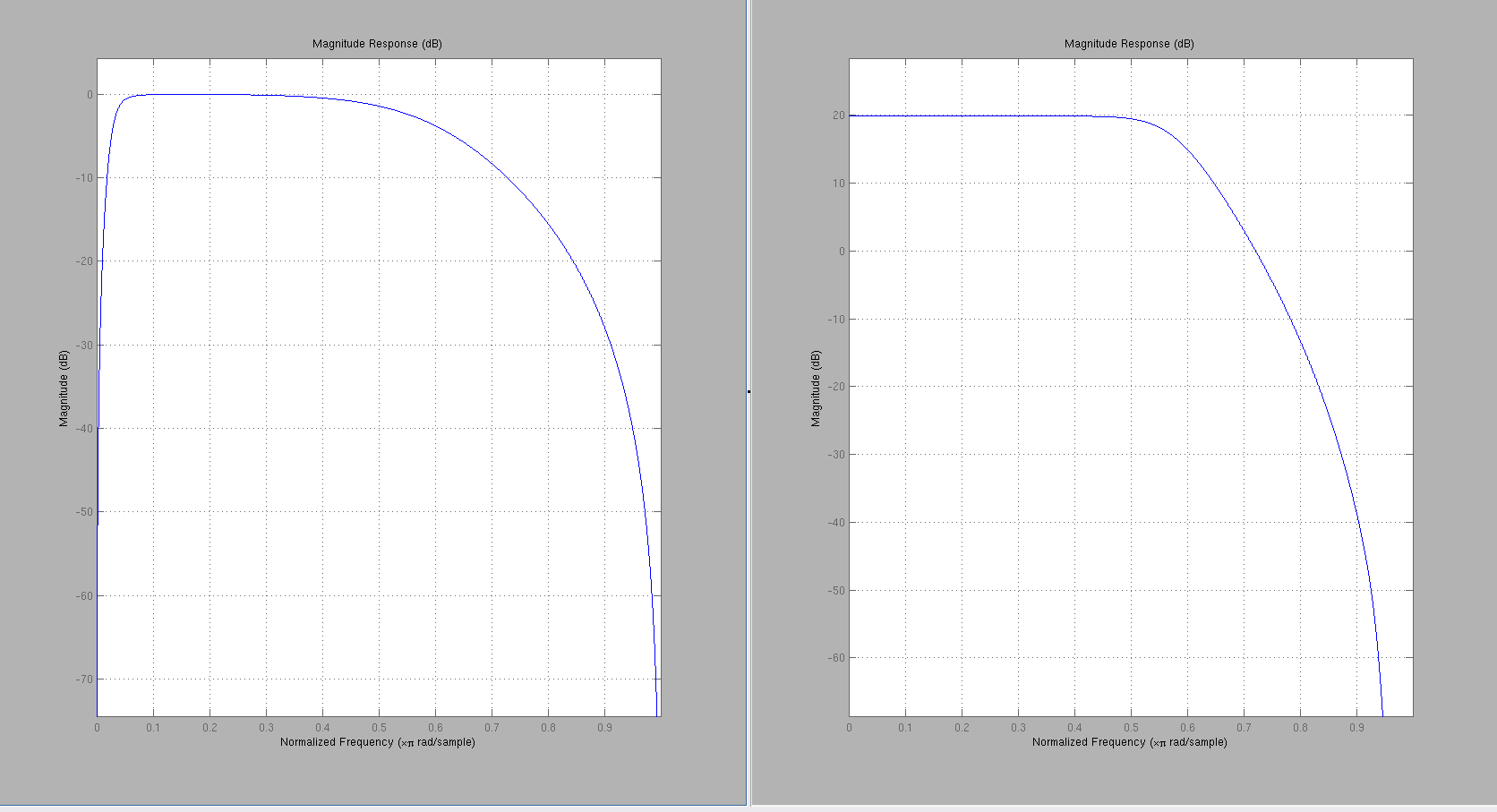
Ironically, the filtering behavior looks better for the 4th-order filter generated from Approach 1, shown below left is the 4th-order biquad cascades. Right is the 8th-order biquad (4 of them) cascades from Approach 2.
In the 8th-order filter, the HPF filter disappeared..not sure why?
Edit: 2/4/2016
While comparing the signal quality between RHD- and RHA-headstage, it seems that RHD headstage is more noisy, even in the middle of the passband (FFT analysis of acquired signals). Therefore the extra noise may be due to the more compact board layout?..As a basic attempt to reduce noise, I reduced the pass band from [500Hz, 9kHz] to [500Hz, 7kHz]. This is also accompanied by my Intan passband setup changes, `gtkclient.cpp` UI changes, and `headstage.cpp` resetBiquad changes.
Original bandwidth settings
Intan cutoff freq: [250Hz, 10kHz]
Intan DSPen setting: High pass above 300Hz
Firmware AGC highpass: > 225Hz
IIR setting: [500Hz, 9kHz]
LPF: b0=6004, b1=12008, a0=-4594, a1=-3039
HPF: b0=15260, b1=-30519, a0=30442, a1=-14213
Reduced bandwidth settings
Intan cutoff freq: [250Hz, 7.5kHz]
Intan DSPen setting: High pass above 300Hz
Firmware AGC highpass: > 225Hz
IIR setting: [500Hz, 7kHz]
LPF: b0=4041, b1=8081, a0=3139, a1=-2917
HPF: b0=15260, b1=-30519, a0=30442, a1=-14213
Edit: 4/6/2016
During [validation](/2016/03/WirelessValidationMetrics) of recording and sorting quality between RHA-headstage, RHD-headstage, and plexon, a few changes to the final deployement firmware was made. Specifically, AGC was replaced by a fixed gain stage. The filtering settings were changed as well.
We widened the Intan’s hardware filter bandwidth so when sorting, the incoming waveform is less distorted and we can better see the spike features. The two stage IIR filters (2 poles on each side) are sufficient to attenuate the undesired out-of-band signals.
Edit: 7/26/2017
After implementing LMS, the input to IIR stage is much less noisy. Keeping the filter bandwidth setting the same – [250, 9kHz], IIR gain makes the spikes much easier to see. RHD headstages have comparable performance to RHA headstages, upon qualitative evaluation (heh).
We want to be able to acquire signals from as many channels as possible. The original headstage Tim designed has four Intan RHA2132 amplifiers, each of which can amplify signals from 32 channels. Based on signals sent to the chip, the internal multiplexer can be instructed to output the analog signals from any of the 32 channels. These measured voltage signals are then passed to 12-bit ADC running at 1MHz, which means each channel is sampled at about 31.25kHz, standard for neural signal acquisition.
The ADC then sends out the conversion results in a serial interface that is compatible with several standards, such as SPI, QSPI, MICROWIRE, as well as Blackfin’s SPORT interface.
This is great news because with the SPORT interface, there are 4 sets of buses available, meaning the blackfin can talk to four ADCs, and therefore sample from 4 RHA2132 channels at time. Meaning we can sample 128 channels at 31.25kHz each.
Further, since RHA2132 acts as simply analog amplifier, communication between the blackfin and RHA2132+ADC is simple:
Receive frame sync (RFS) provides the \(\bar{CS}\) signal to the ADC.
Receive serial clock (RSCLK) provides the SCLK signal to the ADC.
Receive data lines are connected to the ADC’s data output.
The input of the ADC connects to MUXout of RHA2132.
The \(\bar{reset}\) and step signal of all RHA2132 connects to two GPIO pins on the blackfin.
Therefore, at the beginning of each call to DSP-routine, the data values are collected from the SPORT receive buffer. The step line is toggled to step all of the RHA2132’s mux to the next channel. The pin out of this setp is (ADC or amp to blackfin)
Amplifier 1:
ADC1 SCLK - RSCLK0
ADC1 \(\bar{CS}\) - RFS0
ADC1 DATA - DR0PRI
Amp1 \(\bar{reset}\) - PF7
Amp1 step - PF8
Amplifier 2:
ADC2 SCLK - RSCLK0
ADC2 \(\bar{CS}\) - RFS0
ADC2 DATA - DR0SEC
Amp2 \(\bar{reset}\) - PF7
Amp2 step - PF8
Amplifier 3:
ADC3 SCLK - RSCLK1
ADC3 \(\bar{CS}\) - RFS1
ADC3 DATA - DR1PRI
Amp3 \(\bar{reset}\) - PF7
Amp3 step - PF8
Amplifier 4:
ADC4 SCLK - RSCLK1
ADC4 \(\bar{CS}\) - RFS1
ADC4 DATA - DR1SEC
Amp4 \(\bar{reset}\) - PF7
Amp4 step - PF8
Therefore the SPORT ports only receive. SPORT0 generates internal frame sync which becomes the external framesync for SPORT1. The SPORT configurations are (in headstage_firmware/main.c and headstage_firmware/radio5.asm).
1
2
3
4
5
6
7
8
9
SPORT0_RCLKDIV=1SPORT0_RFSDIV=19SPORT0_RCR1=0x0603// early frame sync, active high RFS, require RFS for every wordSPORT0_RCR2=0x010FSPORT1_RCLKDIV=1SPORT1_RFSDIV=19SPORT1_RCR1=0x0401// require RFS for every wordSPORT1_RCR2=0x010F
The RFSCLK is set to be \(\frac{SCLK}{2x(1+SPORTx\_RCLKDIV)}=\frac{80MHz}{4}=20MHz\). Setting SPORTx_RFSDIV=19 means the ADC’s chip select is pulsed high every 20 SCLK cycles for 1 clock cycle. Therefore the ADC is operated at 1MHz. The ADC outputs 12-bits word. There are 20 clock cycles between each chip-select high pulse, thus there are enough clock cycles for the SPORT to read the data output.
This is straight forward and works well.
New implementation with RHD2132
Intan RHD2132 is essentially RHA2132 with a 16-bit ADC built in. The ADC has maximum sampling frequency of 1MHz, which means when the 32 channels are multiplexed, we can achieve 31.25kHz sampling frequency on each channel.
However, RHD2132 needs to interface with other chips through strictly SPI. This introduces two complications:
Instead of simply toggling a pin to reset the amplifier and step the amplifier channel the internal ADC is sampling, each conversion needs to be initiated by a conversion command. This means if we were to keep using the SPORT ports for communication, we have to transmit at the same time as receiving.
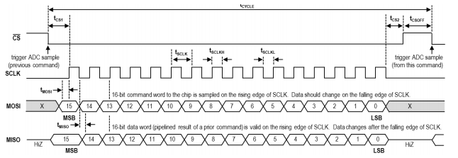
The SPI timing requirement is shown in the diagram below:
The _CS (\(t_{CS1}\)) high duration needs to be greater than 154ns. The datasheet mentions that the _CS line must be pulsed high between every 16-bit data transfer. Finally, \(t_{CS1}\) and \(t_{CS2}\) must be greater than 20.8ns.
The first modification is easily taken care of – we just need to enable the use of SPORTx_TX ports to send Intan commands at the same time as receiving conversion data.
Fulfilling all of the SPI timing requirements is impossible with the SPORT interface because:
RHD2132 transmits and receives only when _CS is pulled low. That means both RFSync and TFSync which dictates when a 16-bits word is received by or transmited from the blackfin, must be connected to _CS, and have the same timing. This was easily done by having TFSync to be internally generated, and set RFSync as externally generated and receives TFSync. The RSCLKx and TSCLKx, which dictates when a bit is sampled or driven out onto the bus is edge-sync’d to the RFSync and TFSync signal, respectively. At the same time, RSCLKx and TSCLKx have to be set to have the same timing, and connects to RHD2132’s SCLK.
The new Blackin SPORT to RHD2132 amplifiers connections are (amplifiers numbered from left to right):
Amplifier 1: SPORT1_SEC
SCLK+ to SCLK1
\(\bar{cs+}\) to FSync1
MOSI+ to DT1SEC
MISO+ to DR1SEC
Amplifier 2: SPORT1_PRI
SCLK+ to SCLK1
\(\bar{cs+}\) to FSync1
MOSI+ to DT1PRI
MISO+ to DR1PRI
Amplifier 3: SPORT0_SEC
SCLK+ to SCLK0
\(\bar{cs+}\) to FSync0
MOSI+ to DT0SEC
MISO+ to DR0SEC
Amplifier 4: SPORT0_PRI
SCLK+ to SCLK0
\(\bar{cs+}\) to FSync0
MOSI+ to DT0PRI
MISO+ to DR0PRI
where SCLK0 is RSCLK0 and TSCLK0 tied together, SCLK1 is RSCLK1 and TSCLK1 tied together, FSync0 is RFS0 and TFS0 tied together, and FSync1 is RFS1 and TFS1 tied together.
This means the falling edge of _CS always corresponds to either the falling/rising edge of SCLK, and similarly, the rising edge of _CS corresponds to either the falling/rising edge of SCLK. However, \(t_{CS1}\) defines the timing between falling edge of _CS and the next rising edge of SCLK, while \(t_{CS2}\) defines the timing between falling edge of _CS and the next rising edge of SCLK. Given the operation of SPORT, one of these requirements will be violated.
My final SPORT settings are, collected from headstage2_firmware/main.c and headstage2_firmware/intan_setup_test.asm (but also other firmware versions. intan_setup_test is simply the first time I tested them):
// SPORT0 transmit// Using TCLK for late-frame syncSPORT0_TCLKDIV=1;SPORT0_TFSDIV=3;SPORT0_TCR2=TXSE|0x10;// allow secondary, 17 bits wordSPORT0_TCR1=TCKFE|LATFS|LTFS|TFSR|ITFS|ITCLK|TSPEN|DITFS;// SPORT1 transmitSPORT1_TCLKDIV=1;SPORT1_TFSDIV=3;SPORT1_TCR2=TXSE|0x10;// allow secondary, 17 bits wordSPORT1_TCR1=TCKFE|LATFS|LTFS|TFSR|ITFS|ITCLK|TSPEN|DITFS;// SPORT0 receive// Serial clock and frame syncs derived from TSCLK and TFS, so RCLKDIV and RFSDIV ignoredSPORT0_RCR2=RXSE|0x10;// allow secondary, 17 bits wordSPORT0_RCR1=RCKFE|LARFS|LRFS|RFSR|RSPEN;// SPORT1 receive// Serial clock and frame syncs derived from TSCLK and TFS, so RCLKDIV and RFSDIV ignoredSPORT1_RCR2=RXSE|0x010;// allow secondary, 17 bits wordSPORT1_RCR1=RCKFE|LARFS|LRFS|RFSR|RSPEN;
In this setup, the receive clock and frame sync are the same as the transmit clock and frame sync. The TSCLK=RSCLK=SCLK of RHD2132, is again set to be 20MHz.
LTFS sets the frame sync signal to be active low.
SPORTx_TFSDIV=3 would mean the frame sync or _CS is pulled low for 1 SCLK (50ns) every 4 cycles (200ns).
However, LATFS sets late frame sync, which means when a frame sync triggers transmission or reception of a word, it will stay low during that time, and another further frame-sync during this time is ignored by the SPORT. After that time, if it’s not time for another frame sync yet, frame sync will return to high, otherwise, it will be low again. Late frame sync also means the timing requiring between the falling edge of _CS and the next rising edge of SCLK is fulfilled.
Together, this means _CS will be low for 17 SCLK cycles, or \(17\times50ns=850ns\) while high for 3 SCLK cycles, or \(3\times50ns=150ns\). This is because, when frame sync first goes low, it will stay low for 17 SCLK cycles, at which time it will go high because 17 is not a multiple of 4. The next greatest multiple of 4 is 20, which is when frame sync will be pulled low again.
The reason for _CS to be low for 17 SCLK cycles is two fold:
Because a dataword is 16 bits, it has to be at least greater than 16 cycles. No matter what settings I have, the \(t_{cs2}\) requirment will be violated, which based on how multiplexer work, will affect the value of the last bit being read. Since the data is read MSBit first, having 17 clock cycles would mean only the 17th bit, which I will discard later will be corrupted by the \(t_{cs2}\) violation. Therefore no harm done!
With _CS low for 17 cycles and high for 3 cycles, I get exactly 20 cycles period, making it 1MHz. This is one of the only configurations that allows me to achieve that.
With this setup, the \(t_{cs2}\) timing requirement is not fulfilled at all, while \(t_{csoff}\) is violated by 4ns.
Initial testing required checking the acquired sample values. Fortunately, all RHD2132 comes with registers that contains the ASCII values of ‘I’, ‘N’, ‘T’, ‘A’, ‘N’. Therefore, if the SPI emulation actually works, I can just issue READ commands of those register locations to Intan, and check whether the received results are correct.
One thing to remember is that when a command to convert a channel is sent, the conversion result is not received until two SPORT cycles later. This also means, if the pipeline is full, when you stop sending commands, it takes two cycles for the pipeline to be completely empty of new data. But since with the SPORT setup, we can’t read from Intan without also sending, that means the last (old) command will have to be send three times during the time it takes to clear the pipeline.
After establishing that, I then needed to make sure I can sample and obtain correct waveforms. This is done by applying a sinusoid of known frequency to the amplifier. In the firmware, I would simply read the the channels four at a time (ch1 on all four amps, then ch2 on all four amps, so on), while sending commands to tell the amplifiers to convert the next channels at the same time as reading. I would save the sample read from the same amplifier every time.
Running this test program (first version is headstage2_firmware/intan_setup_test.asm) and setting breakpoint at the end of execution through JTAG, I can dump the saved data and plot them (using headstage2_firmware/plot_memdump.py).
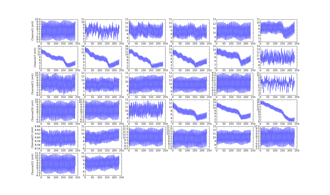
Initial test result for all 32 channels of amplifier 1, when the first channel is applied a 6400Hz signal looks like below:
I have signal, but it’s not what I expected at all…channels without signals are oscillating, there were too many cycles, etc.
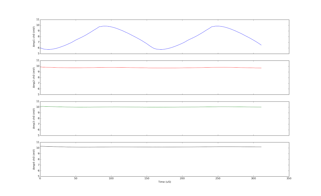
This is strange because when I repeatedly convert just one channel using the same setup (sending CONVERT(0), CONVERT(0)…) rather than converting each channel in turn (sending CONVERT(0), CONVERT(1), CONVERT(2),…), I get great result:
I got two periods on the first channel of amplifier 1. The bottom 3 are the first channels of the other amplifiers, which are quiet as expected.
Turns out the difference is due to reduce sampling frequency. In the second case, where the sampling frequency is 1MHz, each period of 6400Hz wave would require 156 samples.
However, while calculating how many samples I needed to collect in the first case, I mistakenly used the 156 samples/value. When I sample 32 channels round-robin style, the effective sampling rate applied to each channel is 31.25kHz, that means only 5 samples/period is needed. This is why my plots had way more periods than expected.
Secondly, the channels that weren’t applied signals were left floating. This means it’s susceptible to all the noise within the amplifier and PCB planes, resulting in same oscillation frequency, but different amplitude and DC value.
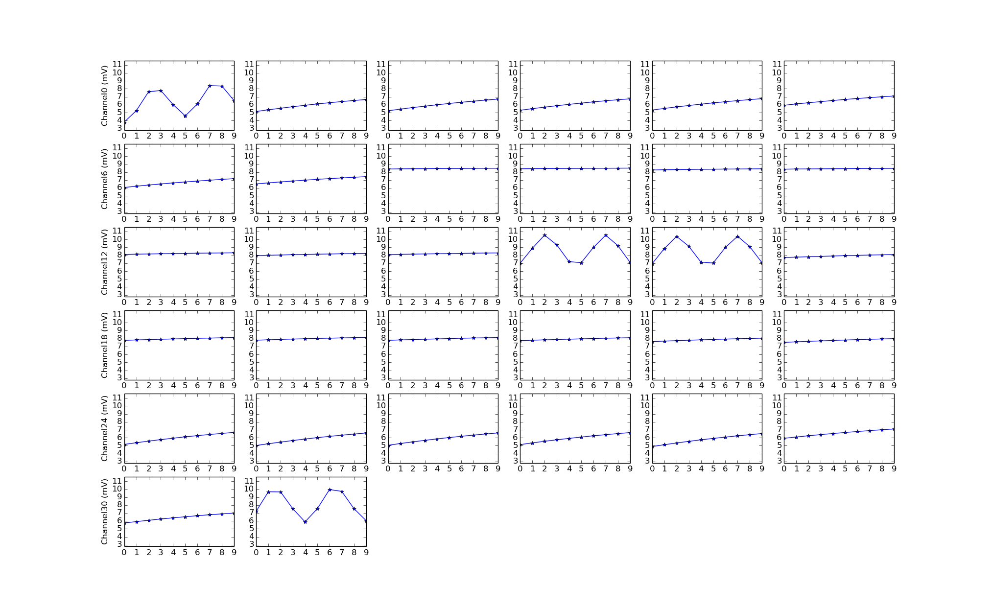
After calculating the correct number of samples to collect to see 2 periods of 6400Hz on all 32 channels of an amplifier, and correctly grounding the channels without applied signals, and turning on Intan’s DSP highpass filter/offset removal, the results then looked just as expected:
In the plot above, channel 0, 15, 31 and 16 are applied the 6400Hz signal while the others are grounded.
Consequences of the new configuration
RHD2132 also support outputting ADC results in either unsigned offset-binary where reference electrode voltage has the value of 0x8000, or using signed two’s complement, where the reference electrode has the value of 0x0000 and values less than that has the MSB set to 1 two’s complement style.
This would result in modifications of the first stage of the firmware’s signal chain, which is to convert the incoming samples to fixed-point Q1.15 format for further processing. See the post on modifying the AGC stage.
Finally, the option DITFS make the SPORT frame-sync, read and write happen every \(1\mu s\) regardless if new commands have been pushed into the SPORT transmit FIFO. This means, if our code-path (signal-chain plus the radio transmission code) inbetween SPORT FIFO reads/writes is too long, the previous command in the FIFO will be sent again, and two cycles later, the corresponding result will be read. This will then result in erroneous data.
However, the manifestation of this data corruption is somewhat counter-intuitive. After establishing correct Intan and SPORT setup to successfully acquire signals, I added in minimally modified signal-chain code from RHA-headstage’s working firmware headstage_firmware/radio5.asm, and saved all pre-processed samples from one of the amplifiers in memory (headstage2_firmware/firmware1.asm). I then stopped the execution when the designated buffer is memory is full, dumped the results for plotting in JTAG. The plots, which I expected to be smooth sinusoids of the applied signal, were riddled with random spikes.
This cannot be due to the signal-chain code since the samples saved came directly from the SPORT. A second test where I simply added nops inbetween SPORT reads/writes confirms that the data corruption was due to the code-path being too long. However, the number of nops that allowed for glitchless data acquisition is less than the signal-chain length used in radio5.asm. This is very strange, since the timing requirement for both headstage firmware setup is similar – accounting for the radio transmission code, the DSP code has to finish in about 800ns. But somehow the timing budget for the RHD-headstage is significantly less.
In the nop test done in firmware2.asm, it was found I can fit 150 nops. I have yet to figure out why this is the case. Regardless, that means a reduction of the original RHA-headstage firmware is needed to adapt it to RHD-headstage. Since the radio-transmission code must stay the same, this reduction is exclusively on the signal-chain code, which includes:
In each signal-chain iteration 4 samples are acquired, 1 per amplifier, so all 4 must be processed. Blackfin works efficiently with two 16-bit samples at once, so samples from two channels are processed first, then the remaining two samples are processed in the rest of the signal-chain code.
Among these, SAA is required for spike matching. AGC is required because the templates for spike-sorting were made under certain signal power level, AGC is needed to fix the channel’s power level. Therefore, all of LMS and half of IIR are ripped out to reduce code-length.
Update: 7/26/2017
The reduction of available processing cycles kept bothering me, so I tried to see what it is caused by and how I can squeeze more cycles.
Setup Intan communication by writing to its config registers and calibrate the ADC comm_setup.
Go to main loop where signal acquistion and processing interleaves with radio transmission.
In step 3, after getting the latest samples from the SPORT buffers, we increment the channel count, construct a proper request to Intan and send it through SPORT again. The SPORT would presumable output this to Intan headstages simulataneously while reading for new samples from Intan. This is done through:
Turns out if in the Intan-setup phase, prior to the start of signal acquisition, I leave the command for auto-incrementing selected amplifier channel in the SPORT transmission (SPORT1_TX, SPORT0_TX) and delete the above snippet from the signal acquisition code, the same behavior is achieved and I can an extra 57 cycles to work with during step 3. This then allows me to fit the entire LMS step into the firmware.
Why does this happen? Probably because accessing the SPORT ports on the blackfin, takes more than 1 CCLK cycle (1/400MHz=2.5ns), which is the case for all the instructions. The ADSP-BF532 hardware reference section 3-5 mentions that Peripheral Access Bus (PAB) and Memory Mapped Register (MMR) access, which includes SPORTx_TX and SPORTx_RX takes 2 SCLK cycles.
SCLK cycle is set to 80MHz, which is 5 CCLK cycles. The code snippet above takes 4*2=8 SCLK cycles, or 40 CCLK cycles. This is less than the extra 57 cycles I got after deleting them, but I think confirms what I see.
I have been working on improving our lab’s old wireless headstage using Analog Device’s Blackfin BF532, Intan’s analog 32-channel amplifiers RHA2136, and Nordic’s NRF24L01 2.4MHz transceivers.
The improvement is replacing the RHA2136 with Intan’s digital version, RHD2132. There are 4 RHA2136 per headstage in the original headstage, each of which requires a voltage regulator and ADC, both of which can be eliminated when using RHD2132. The resulting (ideally working) board would be half the size.
The PCBs have been made. I originally imagined the firmware changes to be minimal – essentially changing how BF532 would talk to the amplifiers through SPI, while keeping most of the signal chain code constant. The code architecture should not have to change much.
However, it has proved to be a lot more difficult than the expected plug-and-play scenario. One of the first issues was to first get Blackfins to talk to the Intans correctly via SPORT. Then I ran into the problem where the original signal chain code in between sample conversions were too long and resulted in data corruption. Therefore, I need to pick parts of the signal chain to cut and modify.
This post documents my work to understand and adapt the integrator-highpass-AGC, the first stage of the signal chain.
Background
The general idea of this wireless system is that, we would acquire samples from four amplifiers at the same time, and then do processing on two of theses samples at a time. Signals at the different stages of the signal chain can be streamed to gtkclient - the PC GUI for display and for spike-sorting. The samples are displayed in a plexon-style interface, and templates are made using PCA. These templates are then sent back to the headstage. In the final firmware, at the end of the signal chain, template matching are done using those results, and a match (or a spike) is found if 16 samples on a given channel is within a certain “aperture” of the templates. (The template is a 16-point time-series. Aperture is the L1-norm of the difference between the template and the most recent 16-samples of the current channel)
Because of this, it would be nice to keep the input signal to template matching at a stable level – a signal with the correct spiking shape, but different signal amplitude may not be catagorized as a match. Thus enters Automatic Gain Control (AGC).
Algorithm
The basic idea is that, the user sets a reference level for the signal power. If the signal power is above this reference level, then decrease the front-end gain. If it is below, then increase it. There are all kinds of fancy implementation, including using different attack/release rate (different gain increasing/decreasing rate). In terms of embeded system, I find this thread, and “TI DSP Applications With the TMS320 Family, Theory, Algorithms and Implementations Volume 2” (pages 389-403) to be helpful in understanding how it works.
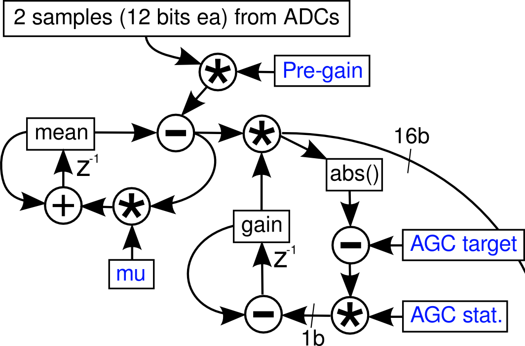
Four samples from each of the 4 ADCs are read at once; as the blackfin works efficiently with two 16-bit samples at once, two samples (from two of the 4 headstages) are then processed at a time. These two come in at 12 bits unsigned, and must be converted to 1.15 signed fixed-point, which is done by pre-gain (usually 4) followed by an integraotr highpass stage. The transfer function of the high pass stage is H(z)=4(1-z^-1)/(1-z^-1(1-mu)); the normal value of mu is 800/16384 […] This is followed by an AGC stage which applies a variable gain 0-128 in 7.8 fixed-point format; the absolute value of the scaled sample is compared to the AGC target (stored as the square root to permit 32-bit integers) and the difference is saturated at 1 bit plus sign. This permits the gain to ramp from 0 to 127.999 in 2^15 clocks.
The accompanying diagram is shown below:
Below is the firmware related to this part - it is obvious now I understand how it works, and Tim’s thesis explanations now makes perfect sense (it did before, but they seemed more like clues to an elaborate puzzle).
//read in the samples -- SPORT0
r0 = w[p0] (z); // SPORT0-primary: Ch0-31
r1 = w[p0] (z); // SPORT0-sec: Ch32-63
r2.l = 0xfff;
r0 = r0 & r2;
r1 = r1 & r2;
r1 <<= 16; //secondary channel in the upper word.
r2 = r0 + r1;
//apply integrator highpass + gain (2, add twice)).
r5 = [i0++]; //r5 = 32000,-16384. (lo, high)
.align 8
a0 = r2.l * r5.l, a1 = r2.h * r5.l || r1 = [i1++]; // r1 = integrated mean
a0 += r2.l * r5.l, a1 += r2.h * r5.l || r6 = [i0++]; //r6 = 16384 (0.5), 800 (mu)
r0.l = (a0 += r1.l * r5.h), r0.h = (a1 += r1.h * r5.h) (s2rnd);
a0 = r1.l * r6.l , a1 = r1.h * r6.l; //integrator
r2.l = (a0 += r0.l * r6.h), r2.h = (a1 += r0.h * r6.h) (s2rnd)
/*AGC*/ || r5 = [i1++] || r7 = [i0++]; //r5 = gain, r7 AGC targets (sqrt)
a0 = r0.l * r5.l, a1 = r0.h * r5.h || [i2++] = r2; //save mean, above
a0 = a0 << 8 ; // 14 bits in SRC (note *4 above), amp to 16 bits, which leaves 2 more bits for amplification (*4)
a1 = a1 << 8 ; //gain goes from 0-128 hence (don't forget about sign)
r0.l = a0, r0.h = a1 ; //default mode should work (treat both as signed fractions)
a0 = abs a0, a1 = abs a1;
r4.l = (a0 -= r7.l * r7.l), r4.h = (a1 -= r7.h * r7.h) (is) //subtract target, saturate, store difference
|| r6 = [i0++]; //r6.l = 16384 (1), r6.h = 1 (mu)
a0 = r5.l * r6.l, a1 = r5.h * r6.l || nop; //load the gain again & scale.
r3.l = (a0 -= r4.l * r6.h), r3.h = (a1 -= r4.h * r6.h) (s2rnd) || nop; //r6.h = 1 (mu); within a certain range gain will not change.
.align 8
r3 = abs r3 (v) || r7 = [FP - FP_WEIGHTDECAY]; //set weightdecay to zero to disable LMS.
r4.l = (a0 = r0.l * r7.l), r4.h = (a1 = r0.h * r7.l) (is) || i1 += m1 || [i2++] = r3;
//saturate the sample (r4), save the gain (r3).
Line 2-8 stores the 12-bit samples in the LO and HI 16-bits of r2.
Line 13 and 14 implement the pre-gain. r5.l=32000=0x7d00 is 0.9765625 in Q15. Multiplying a 12-bit number by 0x7d00 in blackfin’s default mode is equivalent of converting the 12-bit UNSIGNED sample into signed Q15 format. This IS VERY IMPORTANT as I shall see later. Line 14 does it again and then add to the original result. This means by line 15, a0 and a1 contains the original samples multiplied by 2 (although r5.l should really be 0x7fff, which is closer to 1 than 0x7d00 in Q15).
Line 15: r1.l=integrated mean, r5.l=-16384=(Q15) -0.5. The multiply-accumulate (MAC) mode is s2rnd. So, in algebraic form, at the end of the instruction, a0=2x-0.5m[n-1]. r0.l=2*a0=4x-m[n-1]. Here x is the incoming sample, and m[n-1] is the previous integrated mean. Note that since x is 12-bits, then a0 and r0 are at most 14-bits, therefore still positive in Q15 format. Finally, r0 here is actually the output of the integrator-highpass stage (call it y), as also indicated by the diagram.
Line 16: As the comment hints, loads 0.5*m[n-1] into the accumulator. Both numbers are in Q15, the result in the accumulator is Q31.
Line17: From line 15, we have r0=4x-m[n-1]. r6.h=mu=800=(Q15)0.0244140625, which is a constant used to get the desired high-pass response. At the end of this instruction, a0=0.5m[n-1]+mu(4x-m[n-1]).
Since the 40-bit accumulator value is extracted into r2 with (s2rnd) mode, we have r2.l and r2.h to be
2(0.5m[n-1]+mu(4x-m[n-1]))=m[n-1]+2mu(4x-m[n-1]).
As the comment in line 20 hints, this is the new mean.
To characterize the behavior of this integrator-filter stage, we have the following two equations:
\[\begin{align}
m &= mz^{-1}(1-2\mu)+8\mu x \\\\
y &= 4x-mz^{-1}
\end{align}\]
where m is integrated mean, 1/z is delay, x is the original 12-bit samples, y is the output. Note again that since x is 12-bit unsigned, conversion into Q15 does not change anything, therefore the system equations are easy to derive:
The gain is 4, and the 3dB point is determined by \(z=1-2\mu\). In the code \(\mu\approx 0.0244\), so \(z=0.9512\). Note also, in Tim’s thesis, \(\mu\) is actually \(0.0488\), this is because (s2rnd) was used in the actual implementation.
The -3dB frequency can be calculated by plugging in the transfer function into MATLAB, since there’s no easy way to get the Bode plot of a z-transform from the poles and zeros like the analog systems..unless if substituting \(z=exp{j\omega}\) into the transfer function and calculating the magnitude response is easy..
This will plot the two-sided magnitude response. We only care the part where normalized frequency is from 0 to 1. The normalized frequency \(\omega_c\) at the -3dB point can be found be estimated from the plot. Convert to Hz via \(f_c=\omega_c*\pi*F_s/(2*\pi)\). For this AGC setting, \(f_c\approx 225Hz\).
Line 20-23 is the first step of AGC, and is pretty tricky. r5 contains the AGC gain, which as described in the thesis is Q7.8 format (really Q8.8, but we never have negative gain here).
Line 20 multiplies r0 with the AGC gain. But the default mode of multiplication treats both numbers as Q15 fractions, the value inside the accumulator is Q31 and will not be correct. In Q31, the decimal point is after bit 31. But when a Q15 number multiplies a Q7.8 number, there are 15+8=23 fractional bits, and the decimal point is in fact after bit 23.
Therefore, before we can extract the resulting 16-bit number in line 23 (MAC to half-register), we have to shift the results in accumulator by 8. Since the default extraction option takes bit 31-16 after rounding, we get the correct 16-bit results. One questions might be, the result of Q15 and Q7.8 multiplication also have 9 integer bits. In the shift-and-extraction operation, we are essentially throwing away 8 of these integer bits. Turns out the gain is never very big for this to matter (in other words, Q7.8 gives a big range of available gain, but this range is probably not needed).
Finally, r0 in line 23 is the output of the AGC stage.
Important to note here r0 in line 20 is the difference between the new samples and the previous integrated mean, therefore when we take the absolute value of the accumulators in line 21 and line 23, we are essentially getting a measurement of the sigal envelope’s amplitude. And the goal of AGC is to adjust the gain so the signal envelope stays within a target range. This is a very important point. Since Intan implements a highpass DSP filter onboard, I initially thought I could skip the integrator-highpass stage, and plug in the AGC code directly to process the incoming samples. But I simply got rubbish, because the instanteous signal value is not a good measurement of the signal power. The integrator is required to obtain the mean and for this specific AGC implementation to work.
Line 25 does a clever bit of MAC trick. a0 contains the difference of the signal level and the target level. Note that the target level is stored in memory as the square root of the value. Using the (is) mode treats both all numbers involved as signed integer, and the extraction will either be 0x8000 or 0x7fff, for a negative or positive difference. This is significant since 0x8000 and 0x7fff are respectively the smallest negative number and greatest positive number that can be represented in Q15, and allows us to update our AGC gain without doing any if-statement style conditions.
In line 26, r6.h=1 is not the value of mu, but simply indicates whether we have enabled AGC.
Line 27 and line 28 involve yet another fixed-point trick. These two lines updates the AGC gain. The AGC gain in r5 is loaded into the accumulator by multiplying 0x4000 (16384). Afterwards, the MAC with s2rnd option subtract either 0x8000 or 0x7fff from it. This whole procedure is the equivalent of either adding \(2^{-8}\) or subtracting \(2^{-7}\) from the Q7.8 value of the original AGC gain.
The key is noticing that multiplying a Q7.8 number by 0x4000 while treating both as Q15 numbers, then extracting the resulting Q31 number in s2rnd mode, results in a 16-bit number that has the same Q7.8 value as before. This can be demonstrated by the following lines using functions defined in AGC_sim.py:
1
2
3
4
5
gain=52# original gain
Q8_gain=int(decimal_to_Q8_8(52),16)acc_val=int(decimal_to_Q1_31(hex_to_Q15(Q8_gain)*hex_to_Q15(16384)),16)final_gain=mult_acc_to_halfReg(acc_val,0,0,'sub','s2rnd')final_gain=hex_to_Q8_8(final_gain)# should be 52 again.
In line 30, we simply take the absolute value of r3, which contains the new AGC gain, just to be safe.
Implementation for Intan
Understanding that the integrator stage is required for the AGC to work was crucial. Initially giving the unsigned 16-bit Intan samples to the AGC stage (starting around line 20), I simply got rail-to-rail oscillations that didn’t make any sense.
Adding the integrator stage, however, still gave me similar results, but less oscillations. The key to solving this is to realize the original code was written to work with 12-bits unsigned samples. I wish this was emphasized more in the thesis, or perhaps I was just too n00b to realize the significance here.
Since the incoming samples from Intan are 16-bits unsigned in offset binary format – reference value is 0x8000, 0 volts would be 0x0000, and VDD is 0xffff, the conversion step in line 13 by multiplying 0x7fff will often result in a negative result. For example, treating both 0x8000 and 0x7FFF as Q15 numbers, the product is close to -1. Thus the result mean would be -2, rather than 0 (since 0x8000 means signal value at reference voltage). Further, this sign flip would result in new values with different amplitude from the original values.
There are two solutions to this problem:
Right-shift the incoming 16-bit unsigned binary offset samples to 12 bits. Do this right after line 8, and the rest of the code stays unchanged. This approach the least changes to the old firmware (of course, line 1-8 need to be altered to work with Intan, but that’s not algorithmic).
RHD2132 is capable of outputting the ADC samples in 16-bit signed, two’s complement format. This would solve the above mentioned problem of inadvertently flipped signs, since the samples will already in Q15 format. But this would also require changing the integrator-highpass stage, to obtain the same behavior. Specifically, in the system function, there is a pre-gain of 4 in front. This is a result of the line 14, and the two s2rnd operations in line 15 and line 17.
Now that our samples are full 16-bits, we do not need the extra gain. This requires changing the coefficient values in:
r5 in line 11: from r5.l=0x7fff, r5.h=0xc000 to r5.l=0x7fff, r5.h=0x8000.
r6 in line 14: from r6.l=0x4000, r6.h=800 to r6.l=0x7fff, r6.h=1600.
In addition to deleting the accumulator instructions in line 14, and changing the MAC option from (s2rnd) to default in line 15 and line 17.
I ended up using the second approach, because I don’t like throwing away bits. But both works.
**Edit: 4/6/2016
After validation of recording and sorting quality between RHA-headstage, RHD-headstage, and plexon, it looks like AGC amplifies noise too much under low SNR conditions.
As a result, the final deployment firmware uses a fixed pre-gain stage before the IIR stage. This gain is Q7.8 value and can be set in the appropriately compiled version of gtkclient in 0.5 increment from -128 to 127.5.
This book chapter/review paper seeks to tie up a bunch of Shenoy lab work (mostly Churchland) on premotor cortex together with a dynamical system hypothesis - the optimal subspace hypothesis. Central question is what are the neural processes that precede movement and lead to the initiation of movement? And what links movement preparation and movement generation.
The experiment used to derive all the results here is a instructed-delay task, where a monkey first holds its hand in the center, a target then appears, then a go-cue appears, at which the monkey moves to the target.
They first noticed that delay time (between target appearnce and go-cue) is inversely proportional to the reaciton time (time between go-cue and movement-onset). This is hypothesized as a result of more time for movement preparation. So they recorded from the premotor cortex (PMd) and M1, and found activity changes there during the delay period, and seek to find how activties there (indvidual neuron changes vary) contribute to the reduction in movement delay.
(Seems like they are begging the question in terms of which cortical areas to focus on. They mentioned a number of areas show changes in activity during the delay period, yet focus only on PMd and M1. Probably because they only have implants there. Contributions of specific cortical areas to movement preparation is then unclear)
Optimal Suspace Hypothesis
If approaching this question from a dynamical systems perspective, then they will have to answer:
How the activity of a neural population evolves and achieves the needed preparatory state?
How this preparatory state impacts the subsequent arm movement?
What are the underlying dynamics of the neural circuit?
Their solution to the delay period-RT observation is to hypothesis that time is needed for the neural population to achieve some kind of preparatory state which is neccessary for the subsequent movement. Seems like a reasonable hypothesis to me. Specifically, the motor preparation may be the act of optimizing preparatory activity so that the generated movement has the desired properties (what these properties are, they have yet to answer at all).
In a dynamical systems framework, they considered, for a given reach, there is presumably some small sub-region of space containing those values of P that are adequate to produce a successful reach. A smooth relationship exist between firing rate and movement (reasonable), therefore, the small subregion of space is conceived of as being contiguous.
This framework would then predict several things that one can test in the lab (although the order of experiments and hypothesis formulation is probably the opposite in practice here…).
A direct corollary of this framework would be that:
If prep activity is equivalent to initializing a traverse to some optimal subspace for the subsequent movement, these activities for different movements must be different. Movements are defined by their kinematic parameters, thus prep activity should be characterized, or tuned, to these different movement parameters as well.
This is presumable true, have yet to read the Messier and Kalasak, 2000 paper.
Other predictions:
Prediction 1: Reach-speed modulation: Preparatory activity should covary with other meanginful aspects of movement, including peak reach speed. Experiment conducted where monkeys were instructed to reach targets with either faster or lower speed, and the neural data during the preparatory period analyzed.
Prediction 2: Reach-speed (trial-by-trial) correlation: Preparatory activity should correlate, on a trial-by-trial basis, with the peak reach speed. This is mainly to demonstrate the smooth mapping between the neural space and movement parameters, such a trial on the slower side within the instructed-fast condition, should be closer to the those found in the instructed-slow condition than the others. Closeness is measured via distance on the (speed, mean-firing-rate) axis.
Prediction 3: Across-trial firing-rate variance (Fano factor) reduces through time: Preparatory activityshould become, through time, quite accurate and therefore quite similar across trials. In other words, at the end of the preparatory period, the neural activity should become constrained inside the optimal subspace for the subsequent movement, this should manifest in the reduction in variance of the neural activity. The metric they used is the Fano factor (seems rather convoluted), need to read the actual method.
Prediction 4-I and 4-II: Lower Fano factor correlation with lower RTs.
Prediction 5: Perturbing neural activity increases RT: Delivering subthreshold electrical microstimulation (how do they define subthreshold here?) at different times prior to the go-cue in PMd, resulted in longer RT if the stimulation was closer to the go-cue. Stimulating M1 impacted RT less. Effect of stimulation was specific to arm movements and produced little increase in saccadic eye movement RT. The results aligns with theory pretty well, but are the shifts in RT significant? Need to reference the actual paper.
Prediction 6: It should be possible to construct single-trial state-space enural trajectories and use them to directly confirm that across-trial firing-rate variability decrease through time. They recorded a bunch of neurons simultaneously and plotted the neural activity trajectories using Gaussian Process Factor Analysis (GPFA) with dimensionality reduction to visualize. The plots look fine, as in the trajectories run around and converge into different subspaces at different stages of the task. But this can also be due to dimension selection. Need to check the GPFA technique.
Prediction 7: Farther and faster along loop reduces RT. This prediction tries to answer how preparatory state at the time of go cue influence subsequent movement. They hypotehsize that this prep state serves as the initial state of a subsequent dynamical system - thus some region of the brain appear to moniotr and wait for this to be true before “pulling the trigger” to initiate movement. When th trigger is pulled, the further along the loop, the lower the RT. They tested this with offline analysis on a trial-by-trial basis, how far along the loop the prep state was, in relation with that trial’s RT. Of course, this would neccessitate the use of the GPFA plotting of the neural trajectories in finding the actual loop.
To really test these predictions however, we really need to monitor the PMd during brain-control tasks - does the Fano factor analysis still hold? Does the RT still vary with the delay period in brain-control? What else do these prep activities tune for? Does the location of the optimal subspace change following learning (Byron Yu’s null hypothesis papers)?
Implications to BMI if this hypothesis turns out to be a good framework: How long does it take for the neural trajectory to change from baseline to the optimal subspace? Can we make decoders detect/classify these spaces? Shenoy suggests 200ms as measured with single-trial neural trajectories as the transition period needed for transition between baseline to the optimal subspace, thus decoding during this period should be avoided (will have to read the paper to evaluate this).
References to Read
Churchland, M. M., Afshar, A., & Shenoy, K. V. (2006a). A central source of movement variability. Neuron, 52, 1085–1096
Churchland, M. M., Cunningham, J. P., Kaufman, M. T.,Ryu, S. I., & Shenoy, K. V. (2010a). Cortical preparatory activity: Representation of movement or first cog in a dynamical machine? Neuron, 68, 387–400
Churchland, M. M., Kaufman, M. T., Cunningham, J. P., Ryu, S. I., & Shenoy, K. V. (2010b). Some basic features of the neural response in motor and premotor cortex. In Program No. 382.2. Neuroscience meeting planner. San Diego, CA: Society for Neuroscience Online
Churchland, M. M., Santhanam, G., & Shenoy, K. V. (2006b). Preparatory activity in premotor and motor cortex reflects the speed of the upcoming reach. Journal of Neurophysiology, 96, 3130–3146
Churchland, M. M., & Shenoy, K. V. (2007a). Delay of movement caused by disruption of cortical preparatory activity. Journal of Neurophysiology, 97, 348–359.
Churchland, M. M., Yu, B. M., Cunningham, J. P., Sugrue, L. P., Cohen, M. R., Corrado, G. S., et al. (2010c) Stimulus onset quenches neural variability: A widespread cortical phenomenon. Nature Neuroscience, 13, 369–378
Churchland, M. M., Yu, B. M., Ryu, S. I., Santhanam, G., & Shenoy, K. V. (2006c). Neural variability in premotor cortex provides a signature of motor preparation. The Journal of Neuroscience, 26, 3697–3712
Messier, J., & Kalaska, J. F. (2000). Covariation of primate dorsal premotor cell activity with direction and amplitude during a memorized-delay reaching task. Journal of Neurophysiology, 84, 152–165.
Santhanam, G., Ryu, S. I., Yu, B. M., Afshar, A., & Shenoy, K. V. (2006). A high-performance brain-computer interface. Nature, 442, 195–198.
Santhanam, G., Sahani, M., Ryu, S. I., & Shenoy, K. V. (2004). In: An extensible infrastructure for fully automated spike sorting during online experiments (pp. 4380–4384). Proceedings of the 26th annual international conference of IEEE EMBS, San Francisco, CA.
Yu, B. M., Afshar, A., Santhanam, G., Ryu, S. I., Shenoy, K. V., & Sahani, M. (2006). Extracting dynamical structure embedded in neural activity. In Y. Weiss, B. Schölkopf & J. Platt (Eds.), Advances in neural information processing systems, (Vol. 18, pp. 1545–1552). Cambridge, MA: MIT Press
Yu, B. M., Cunningham, J. P., Santhanam, G., Ryu, S. I., Shenoy, K. V., & Sahani, M. (2009). Gaussian-process factor analysis for low-dimensional single-trial analysis of neural population activity. Journal of Neurophysiology, 102, 614–635.
Thesis: optimal codesign of decoders and concomitant engagement of neural adaptation is important.
Decoding vs. Learning.
Decoder design begins by (1) training a decoder to predict natural or intended movement from previously recorded open-loop neural data and (2) assumes that the statistics of the neural activity remain the same when controlling the BMI during the closed-oop phase.
Neural adapation approach begins by (1) starting with a decoder that is not trained to predict natural or intended movement, and instead has minimal structure within its decoder paratmers, and (2) takes the view that there is a de novo, closed-loop system that has to be learned by the brain in order to achieve proficient BMI control.
These two approaches do not have to be exclusive.
Three experimental model:
hand-controlled training, hand-free BMI control. No context switch between change, so movement continue from training to BMI. Lead to high performance with biomemtic decoder design.
hand-controlled training, hand-independent BMI control - involves context change between control change. Hand free to move in brain-control. The same movements that were used to train the open-loop decoder cannot be made during BMI. This process predicts more meaningful neural adaptation changes.
hand-constrained training, hand-constrained BMI control without context change via passive observation. Less mismatch between closed-loop BMI operation and open-loop decoder training, can lead to high BMI perforance but predict less neural adapatation.
CLDA e.g. Carmena’s PVKF with Smooth-batch or ReFIT may combine decoder adapation with neural adapation. Requires “intention estimation” which I think is hard to generalize, but it’s also the easiest closed-loop adaptation to implement.
Neuro-adapation allows animals to effectively learn at least a slightly different decoder each day before being able to perform the task proficiently. But this is difficult for more complex task with higher DOF. The key is to pair stable neural populations with fixed, static decoder. Differential modulation of neuronal populations based on their causal link to neuroprosthetic control, resulting netowrks co-existing with native cortical networks, can switch without interference based on task requirements, blablabla nothing new here, just re-iterating the Ganguly-Carmena 2011 paper.
The real challenge is to control two different BMI using two decoder from two separate neural ensembles!
**How do these adapations happen? Basal ganglia? **
Mouse studies (Yin et al., 2009)showed increasing coherence between M1 and dorsostlateral striatum neurons during learning to brain-control using M1 neurons.
Changes in cohereance were temporally precise and significantly more pronounced in direct M1 neurons than in those not controlling the BMI - consistent with formation of a BMI-specific network. Further, knckout mice lacking NMDA receptors in the striatum were not able to learn the same task, supporting the notion that corticostriatal plasticity is necessary for neuroprosthetic learning. Together these results suggest that corticobasal ganglia circuits are invovles in BMI learning, even when they do not require physical movement. [...] neural adapatation not only elicits changes in motor cortical networks, but also recruits elements fo the natural motor system outside of the cortex such as the basal ganglia.
This is pretty cool…brain has so much generalization capability, motor learning is like the greatest API ever for BMI! On the other hand, if BMI learning is so closely coupled with the motor learning process (signaled by the activation of the corticobasal ganglia circuits), would that imply subjects who have more proficient motor learning would also be more proficient at learning different modes of BMI control (at least when using M1 ensembles)?
Can try a bimanual task where one hand is controlled by BMI the other by native arm.
How does the decoder know if the user intends to use the BMI controlled device? Motor cortex is always active and not strictly lateralized and is part of a coordinated bimanual circuit. This correlation may not be readily separated by the decoder, especially if neural activity from both contra- and ipsilateral motor cortex couupy the same neural dimensions.
Thus the onus would then fall on neural adaptation to create a new motor control circuit, which effectively decorrelates control of the intact arm from the prosthetsis, so that the subject can have independent control of both her real and prosthetic limb and hand.
References to Read
Chase, S.M., Kass, R.E., and Schwartz, A.B. (2012). Behavioral and neural correlates of visuomotor adaptation observed through a brain-computer interface in primary motor cortex. J. Neurophysiol. 108, 624–644.
Chestek, C.A., Gilja, V., Nuyujukian, P., Foster, J.D., Fan, J.M., Kaufman, M.T., Churchland, M.M., Rivera-Alvidrez, Z., Cunningham, J.P., Ryu, S.I., and Shenoy, K.V. (2011). Long-term stability of neural prosthetic control signals from silicon cortical arrays in rhesus macaque motor cortex. J. Neural Eng. 8, 045005.
Dangi, S., Gowda, S., Moorman, H.G., Orsborn, A.L., So, K., Shanechi, M., and Carmena, J.M. (2014). Continuous closed-loop decoder adaptation with a recursive maximum likelihood algorithm allows for rapid performance acquisition in brain-machine interfaces. Neural Comput. 26, 1811–1839.
Durand, D.M., Ghovanloo, M., and Krames, E. (2014). Time to address the problems at the neural interface. J. Neural Eng. 11, 020201.
Fan, J.M., Nuyujukian, P., Kao, J.C., Chestek, C.A., Ryu, S.I., and Shenoy, K.V. (2014). Intention estimation in brain-machine interfaces. J. Neural Eng. 11, 016004.
Fetz, E.E. (2007). Volitional control of neural activity: implications for braincomputer interfaces. J. Physiol. 579, 571–579
Gage, G., Ludwig, K., Otto, K., Ionides, E., and Kipke, D. (2005). Naive coadaptive
cortical control. J. Neural Eng. 2, 52–63
Jarosiewicz, B., Masse, N.Y., Bacher, D., Cash, S.S., Eskandar, E., Friehs, G., Donoghue, J.P., and Hochberg, L.R. (2013). Advantages of closed-loop calibration in intracortical brain-computer interfaces for people with tetraplegia. J. Neural Eng. 10, 046012.
Kao, J.C., Stavisky, S., Sussillo, D., Nuyujukian, P., and Shenoy, K.V. (2014). Information systems opportunities in brain-machine interface decoders. Proceedings of the IEEE 102, 666–682.
Koralek, A.C., Jin, X., Long, J.D., II, Costa, R.M., and Carmena, J.M. (2012). Corticostriatal plasticity is necessary for learning intentional neuroprosthetic skills. Nature 483, 331–335.
Koralek, A.C., Costa, R.M., and Carmena, J.M. (2013). Temporally precise cellspecific coherence develops in corticostriatal networks during learning. Neuron 79, 865–872.
Lebedev, M.A., Carmena, J.M., O’Doherty, J.E., Zacksenhouse, M., Henriquez, C.S., Principe, J.C., and Nicolelis, M.A. (2005). Cortical ensemble adaptation to represent velocity of an artificial actuator controlled by a brainmachine interface. J. Neurosci. 25, 4681–4693.
Merel, J., Fox, R., Jebara, T., and Paninski, L. (2013). A multi-agent control framework for co-adaptation in brain-computer interfaces. Proceedings of the 26th Annual Conference on Neural Information Processing Systems, 2841–2849.
Milla´ n, Jdel.R., and Carmena, J.M. (2010). Invasive or noninvasive: understanding brain-machine interface technology. IEEE Eng. Med. Biol. Mag. 29, 16–22
Yin, H.H., Mulcare, S.P., Hila´rio, M.R., Clouse, E., Holloway, T., Davis, M.I., Hansson, A.C., Lovinger, D.M., and Costa, R.M. (2009). Dynamic reorganization of striatal circuits during the acquisition and consolidation of a skill. Nat. Neurosci. 12, 333–341.
Sussillo D, Nuyujukian P, Fan JM, Kao JC, Stavisky SD, Ryu SI, Shenoy KV (2012) A recurrent neural network for closed-loop intracortical brain-machine interface decoders. Journal of Neural Engineering. 9(2):026027
Sensory feedback was achieved by stimulating peripheral nerve fascicles, which, in turn, allowed real-time closed-loop control of a prosthetic hand by a human subject with a transradial amputation. To restore the lost sensory feedback, four TIMEs were implanted in the median and ulnar nerve fascicles, and two stimulation sites that were able to elicit distinct and repeatable sensations on the innervation territories of the two nerves (3–5) were then selected at the end of systematic testing of all the contacts and then connected to the artificial hand sensors. Sensations were elicited in a range from slight contact to just below the reported pain threshold, to dynamically control the intensity of stimulation delivered, according to the prosthetic hand sensor readouts.

The participant controlled the prosthesis through voluntary contractions of the remaining muscles on the stump, being able to perform different (ulnar, pinch, and palmar) grasps, and hand opening by online processing of sEMG signals. The grasps were performed in terms of position control such that he was able to finely modulate the fastening and opening of the prosthetic hand.
The best part is with the nerve stimulation, the subject can distinguish between at least three different shapes, sizes, and stiffness. The stimulation was modulated at 50Hz, biphasic, and only amplitude varied.
Focuses on the acquisition of “neuroprosthetic skill”, performance and neural representations that are robust over time and resistant to interfernce. As shown before, learning in brain-control facilitate the formation of BMI-specific control networks, changes in cortical and corticostriatal plasticity show speficificty for BMI control neurons. Evidence seems to suggest that neuroplasticity creates specialized BMI control network that allows skillful control.
Cortical map formation has been shown to be sensitive to the details of the BMI system, such as the neurons input into the decoder, and decoder parameters. Training new decoders regularly, even with the same neural ensemble, elminated cortical map formation and the associated performance improvement. This would then suggest a fixed decoder would allow neuroplastiicty to yield continued task performance from day to day. However, the decoder’s performance is sensitive to changes in the neural signals. Thus closed-loop adapation can facilitate and maintain learning in the presence of changing neural inputs to the BMI. Therefore the control architecture of closed-loop decoder adaptation (CLDA) as a two-learner system can provide more robust BMI performance.
In the first experiment, a delayed center-out hold task is used. CLDA was used initially to train the decoder (via smooth-batch or ReFIT). CLDA was stopped until the monkey can navigate the cursor across workspace - the goal is to limit decoder adapation to maximize improvement driven by neural adapation, perhaps this allows for more robust neuroprosthetic skill retention?
Performance (measured by % correct, success rate - trials/min, and mean error - deviation from ideal trajectory) continued to improve after the decoders were held fixed. Intermittent CLDA was used to compensate for performance drops and changes in the neural ensemble.
One key finding was that
[…] gradual refinement of cursor control, with continued improvements in movement errors and success rates reached a plateau. These improvements were absent when CLDA was used each day to maximize performance starting from varying initial decoders that used differeint neural ensembles. Whereas CLDA could achieve high task performance, movement kinematics showed no improvements. Daily performance also showed variability commonly observed with daily re-training. This finding confirms that observed learning was not purely reflective of increased practice in BMI and highlights the improtance of some degree of neural and decoder stability for learning.
While the specifics of how CLDA is used exactly in their training scheme are needed for me to accept their conclusion (reseeding CLDA every day would introduce abrupt changes to the decoder, as the authors mention), but the idea of intermittent decoder adapation and neural plastiticty can be useful. Also supports using reinforcement learning to train the decoder…
Neural data analysis:
Tuning map correlate strongly in later sessions, less tuning changes in later sessions indicate saturation.
Degree of neural adaptation depends on amount of performance improvements - correlation of tuning maps with day 1 decrease with sessions and performance rate. Really just a corrollary of analysis 1.
Neural adapation is shaped by decoder properties - tuning properties changed primarily when necessary to improve performance and otherwise stable. Specifically, units were more likely to change their preferred directions if the initial decoder assigned them an “incorrect” PD. If they did the same analysis on the Ganguly, Carmena 2011 paper on direct and indirect neuron populations, would they still reach the same results with the direct neuron population? What about the indirect neurons?
They compared the onset time of directionally tuned activity and time of peak firing for each unit during different sessions. Averaging across all units and series, they found that after learning:
units were both directionally tuned earlier and reached peak firing earlier in the trial (Wilcoxon sign-rank test).
Majority of units developed tuning prior to the go-cue - indicate planning or preparation to move.
Cursor speed profiles also shifted earlier with learning, and clear increases in speed occured prior to the go-cue. (WTF the cursor isn’t supposed to move before go-cue!).
Second Experiment
To test the robustness of neuroprosthetic skill and the emerging neural map’s resistance to interference from exposure to other contexts and perturbing neural inputs, specifically, from native motor networks, the BMI-SC task involved the monkey pressing down on a force sensor with arm contralateral to the implants, whlie performing the regular task. The decoder used in BMI-SC and regular BMI task is the same.
Results here include:
Isometric force task significantly disrupted the task performance.
BMI-only performance and learning not disrupted by performing the BMI-SC task in the same day.
Sessions in which BMI-only and BMI-SC tasks were perofrmed in A-B-A block showed minimal within-session interference between contexts, confirms the reversible modification hypothesis from Ganguly, Carmena 2011.
BMI-SC performance also improved across the series, approaching that of BMI-only performance on the last day in one example. These improvements may be due in part to reduced interference of arm-movement-related activity with BMI control, the disruption of simultaneous arm movements may not be fully blocked by skill formation. Learning Transfer between contexts.
Performance improved even when CLDA was used to fully adapt the decoder, suggesting that neural plasticity may provide benefits beyond decoder adapation alone. Gradual adapation might be kye.
References to Read
Collinger, J.L., Wodlinger, B., Downey, J.E., Wang, W., Tyler-Kabara, E.C., Weber, D.J., McMorland, A.J., Velliste, M., Boninger, M.L., and Schwartz, A.B. (2013). High-performance neuroprosthetic control by an individual with tetraplegia. Lancet 381, 557–564
Dangi, S., Orsborn, A.L., Moorman, H.G., and Carmena, J.M. (2013). Design and analysis of closed-loop decoder adaptation algorithms for brain-machine interfaces. Neural Comput. 25, 1693–1731
Gilja, V., Nuyujukian, P., Chestek, C.A., Cunningham, J.P., Yu, B.M., Fan, J.M., Churchland, M.M., Kaufman, M.T., Kao, J.C., Ryu, S.I., and Shenoy, K.V. (2012). A high-performance neural prosthesis enabled by control algorithm design. Nat. Neurosci. 15, 1752–1757
Pretty heavy math, will have to go over this again. Premise is that small changes in closed-loop BMI dynamical properties can have significant and predicatable effects on performance. PVKF was used as a specific algorithm to study.
Two undesired effects:
presence of unintended attractor points which pulled the cursor to arbitrary workspace positions.
calibration-dependent control memory property which parameterized the tradeoff between speed and hold performance. likely driven by fluctuation in the closed-loop control memory of the decoder.
Both properties were not only present in experimental data but also their mathematical causes could be traced back to the mechanics of the closed-loop decoder. For KF, and generally for recursive Bayesian decoders, the closed-loop properties induced by interaction between the sate-space model and the neural firing model can produce unintentional dynamical artifacts.
There are numerous benefits of keeping both the decoder and the neural ensemble fixed across sessions. However, CLDA is needed to adapt to nonstationarity of the ensemble, and initial calibration. But CLDA can also change system properties that one might prefer to keep fixed if one wishes to keep the system as consistent as possible before and after calibration.
References to Read
F. R. Willett , A. J. Suminski , A. H. Fagg and N. G. Hatsopoulos “Improving brain-machine interfaceperformance by decoding intended future movements”, J.Neural Eng., vol. 10, no. 2, pp.026011 2013
B. Jarosiewicz , S. M. Chase , G. W. Fraser , M. Velliste , R. E. Kass and A. B. Schwartz “Functional network reorganizationduring learning in a brain-computer interface paradigm”, Proc. Nat. Acad. Sci., vol. 105, no. 49, pp.19486 -19491 2008
E. J. Hwang , P. M. Bailey and R. A. Andersen “Volitional control of neuralactivity relies on the natural motor repertoire”, Curr.Biol., vol. 23, no. 5, pp.353 -361 2013
W. Wu , Y. Gao , E. Bienenstock , J. P. Donoghue and M. J. Black “Bayesian population decoding of motor corticalactivity using a Kalman filter”, Neural Comput., vol. 18, no. 1, pp.80 -118 2006
Z. Li , J. E. O'Doherty , M. A. Lebedev and M. A. L. Nicolelis “Adaptive decoding for brain-machineinterfaces through Bayesian parameter updates”, NeuralComput., vol. 23, no. 12, pp.3162 -3204 2011
M. Golub , S. M. Chase and B. M. Yu “Learning an internal dynamics model fromcontrol demonstration”, Proc. Int. Conf. Mach.Learn., vol. 28, pp.606 -614 2013
Simple binary BMI-control demonstration with the RLBMI framework. Finally showed some neural data, and showed that the RLBMI approach is robust against neuron loss. They are calling their RL neural decoder in Sanchez 2013 “Associative reinforcement learning that combined elements of supervised learning with reinforcment based optimization”.
Since the experiment control is so simplistic, cannot derive much value about this decoder’s performance compared to other closed-loop based methods. But
The RLBMI maintained high performance when applied in a contiguous fashion across experiment sessions spanning up to 17 days. The decoder weights started from random initial conditiosn during the first session, and during subsequent sessions the system was intialized from wegiths learning in the previous session, and was then allowed to adapt as usual without any new initializations or interventions. […] Half of the neural input signals were lost between day 9 and 16. However, the system was able to quickly adapt and this loss resulted in only a slight dip in performance.
References to Read
Ludwig KA, Miriani RM, Langhals NB, Joseph MD, Anderson DJ, et al. (2009) Using a common average reference to improve cortical neuron recordings from microelectrode arrays. J Neurophysiol 101: 1679–1689. doi: 10.1152/jn.90989.2008
Schultz W (2000) Multiple reward signals in the brain. Nat Rev Neurosci 1: 199–207. doi: 10.1038/35044563
Theory paper toward which the Sanchez guys have been working toward. The RLBMI decoder architecture is now presented as an actor-critic method of RL, where the neuroprosthetic controller (actor) learned the neural state-to-action mapping based on the user’s evaluative feedback. The role of teh critic is to translate the user’s feedback into an explicity training signal taht can be used by the factor for adaptation. The aim is to learn and automatically produce a stable neural to motor mapping and respond to pertubations by readjusting its parameters in order to maintian the performance, using a binary evaluative feedback. The metrics for the controller’s performances used were:
speed of convergence.
generalization
accuracy and recovery from perturbation
Reinforcement Learning, control architecture, learning algorithm - Instead of using Q-learning with a NN to act as the action-reward mapping, a Hebbian reinforcement learning framework is used. I’m confused as to why this group decided to switch the RL-framework. I am not very familiar with all the ML techniques yet, but according to scholarpedia, we need to distinguish between the machine learning/TD-learning […] and the neuronal perspective. The machine learning perspective deals with states, values, and actions, etc., whereas the neuronal perspectives tries to obtain neuronal signals related to reward-expectation or prediction-error. Regardless, the basic strategy is the same: initialize a random decoder, based on some feedback on whether the decoded action is correct or not, update the NN weights. With more trials, both the decoder and the user adapt toward each other.
Tasks
The sequential mode is where the controller has to perfrom a sequence of actions over mulitple steps in order to accomplish the goal of a trial. This means that there can be multiple sequences of actions that could eventually result in the end goal, and thus mulitple solutions that could be learned by the HRL. Reward/feedback is received by the controller after every action. The metric for reward in movement given in this paper is whether a specific time-step the action moves the manipulandum closer towards the targe.
But I can imagine this approach suffering from the problem common to some greedy algorithms - sometimes the greedy approach might not give the optimal solution. Also possible that this intention estimation is too constraining - the animal might not actually want to move in the most direct trajectory possible, but this may not be important in terms of BMI for patients, efficiency is probably the most important factor there.
The episodic mode where the controller can select only one action in each trial, and thus that action must achieve the goal for a successful trial. The episoic learning mode is suitable for classification tasks. This is what Sanchez 2011 used for their center-out task. Since achieving the trial goals requires only a signel action here, the HRL can be encouraged to learn more quickly in the episodic task compared to the sequential task. Experience replay can be used to seed learning in this paradigm.
Since the sequential mode is a sequence of actions, using episodic mode to intitialize the decoders for sequential mode can probably speed up the learning process.
Network was first tested in simulation experiments, developed for a reaching task in 2D grid space, useful for validating the actual computational model. Three components:
Synthetic neural data generator, with each neuron tuned to one action (moving left, right, up, and down) or none. Goal of the user is to reach targets in 2D space. Input feature is firing rates in 100ms bins.
Neuroprosthetic controller (actor).
Behavioral paradigm - gives binary feedback to the controller.
Experiments were done in common-marmosets, utilizing a Go/No-Go motor task to move a robot arm to spatial targets to either the left or right side of the monkey. Catch Trial - traning technique to ensure the monkeys understood the necessity of the robot movements where the robot moved in the opposite direction commanded by the monkey and thus the monkey received no reward.
Results
Simulation results showed the the weights converging to achieve high success rates for both tasks, as expected. Robust against neuron loss and tuning changes.
The monkey neural data were used offline to map to four different directions. Complete BS, the analysis makes no sense since the monkey was simply trained to perform Go/No-go arm movement. This is bad.
References to Read
Francis J T and Song W 2011 Neuroplasticity of the sensorimotor cortex during learning Neural Plast. 2011 310737
Heliot R et al 2010 Learning in closed-loop brain-machine interfaces: modeling and experimental validation IEEE Trans. Syst. Man Cybern. B 40 1387–97
Prasad A et al 2012 Comprehensive characterization and failure modes of tungsten microwire arrays in chronic neural implants J. Neural Eng. 9 056015
Polikov V S, Tresco P A and Reichert W M 2005 Response of brain tissue to chronically implanted neural electrodes J. Neurosci. Methods 148 1–18
Mahmoudi B and Sanchez J C 2011 A symbiotic brain-machine interface through value-based decision making PLoS One 6 e14760
Schultz W, Tremblay L and Hollerman J R 1998 Reward prediction in primate basal ganglia and frontal cortex Neuropharmacology 37 421–9
Izawa E I, Aoki N and Matsushima T 2005 Neural correlates of the proximity and quantity of anticipated food rewards in the ventral striatum of domestic chicks Eur. J. Neurosci. 22 1502–12
Wawrzyński P 2009 Real-time reinforcement learning by sequential actor–critics and experience replay Neural Netw. 22 1484–97
Schultz W 2000 Multiple reward signals in the brain Nature Rev. Neurosci. 1 199–207
Prins N et al 2013 Feature extraction and unsupervised classification of neural population reward signals for reinforcement based BMI Annu. Int. Conf. IEEE Eng. Med. Biol. Soc. (EMBC) (Osaka, Japan, 2013) at press
Ribas-Fernandes J J F et al 2011 A neural signature of hierarchical reinforcement learning Neuron 71 370–9
Monitored ensembles of neurons that were either casually linked to BMI control or indirectly invovled, found that proficient neuroprosthetic control is associated with large-scale modifications to the cortical network. […] Specifically, there were changes in the preferred direction of both direct and indirect neurons. Notably, with learning, there was a relative decrease in the net modulation of indirect neural activity in comparison with direct activity. […] Thus, the process of learning BMI control is associated with differential modification of neural populations based on their specific relation to movement control.
Results pretty intuitive, but analysis methods are useful to know.
Experiment
Recorded ensembles of M1 neurons while only a subset were assigned to have a causal role during control as direct neurons. The monkyes performed center-out reaching movements using a exoskeleton that constrained movements to the horizontal plane.
Used a linear decoder for motor commands. Decoder was held constant after initial training. Stability of recordings across days assessed by measuring the stationarity of spike waveforms and the interspike interval distribution, as well as directional modulation during manual control sessions.
Results
Modification of preferred directions
There is a relative remapping of the preferred directions for all neurons without any substantial systematic rotational shifts for each neural opulation.
Differential modification of modulation depths
Direct and indirect neurons had different tuning depth. This differential modulation was specifically present during proficient neuroprosthetic control and not during the initial learning period. At population level, no significant systematic differences in the mean firing rate between manual control and brain control for either populations.
Reversibility of modifications
Modulation depths for the manul-BMI-manul experimental scheme changes, while being similar during the manual sessions. This suggests reversibility in the large-scale modifications dependent on cortical state (manual vs. BMI_
Stability
Indirect neurons maintained a relatively fixed neuron-behavior relationship during brain-control through sessions across days. May suggest an active role to brain-control? Probably related to the irrotational shift of tuning properties.
Used bootstrap resampling methods for testing significance in directional tuning and mean modulation depth changes.
This paper seeks to demonstrate that single units/multiunits and local field potentials in M1 are modulated by reward expectaiton during reaching movements and that this modulation is present even while subjects passively viewed cursor motions that are predictive of either reward or nonreward. They also tried to classify whether a trial is rewarding vs. nonrewarding based on the neural data, on a moment-to-moment basis.
Experiments:
Monkey arm wears an exoskeletal robot through all tasks. Use a single target during all trials
Manual Task. The monkey was required to hold at the center target for 325ms before teh peripheral target appeared, then hold an additional 300ms before the center target disappearted, the go cue appearing for moving to the peripheral target, and hold for 325ms before receiving a liquid reward or no reward.
The paper does not manually control for monkey arm trajectory, speed, etc. But in offline analysis they selected kinematically indistinguishable trajectories between the two reward contingencies to isolate the effect of reward.
OT1. Monkey arm is fixed by the robot and cannot move. The monkey would fixate at the center target and observe the center target change color; red represents a rewarding trial, blue represents a nonrewarding trial. The cursor would then move toward the peripheral target at a constant speed with movement toward a red target resulitng in a reward, once the cursor arrived inside the target. For blue targets, reward was withheld. The monkey had to view the target plane to start a trial and maintain visual gaze until the color cue was given.
OT2. The monkey observed the cursor moving away or twoard a target with movement toward a the target resulting in a reward, once the cursor arrived inside the target. No reward otherwise.
Results:
Some neurons fired higher throughout reward trials, while others behaved the opposite way. Both contralateral and ipsilateral M1 contains units that simultaneously correlat with reward and kinematics during reaching and observation…but how to identify which is reward-modulated in a less controlled BMI experiment?
Classifiers were trained using PCA components to classify reward vs. nonreward trials. The average classifer performance (over trial length) is around 70%, pretty good.
Simulated RL-BMI using TD-learning, NN for action-reward mappings. Works well, not too surprising, but not too much value either with a two-state classification task.
References to Read
Dura-Bernal S, Chadderdon GL, Neymotin XZ, Przekwas A, Francis JT, Lytton WW (2014) IEEE Signal Processing in Medicine and Biology Symposium (SPMB’13) Virtual musculoskeletal arm and robotic arm driven by a biomimetic model of sensorimotor cortex with reinforcement learning
Hosp JA, Pekanovic A, Rioult-Pedotti MS, Luft AR (2011) Dopaminergic projections from midbrain to primary motor cortex mediate motor skill learning. J Neurosci 31:2481–2487.
Legenstein R, Chase SM, Schwartz AB, Maass W (2010) A reward-modulated hebbian learning rule can explain experimentally observed network reorganization in a brain control task. J Neurosci 30:8400–8410.
Todorov E, Jordan MI (2002) Optimal feedback control as a theory of motor coordination. Nat Neurosci 5:1226–1235.
I am a bit puzzled why this paper is published in 2011, after the DiGiovanna 2009, when the experiment less complicated, but with the same premise. I speculate it might be this paper demonstrates RLBMI experiments in rhesus monkeys, instead of rats.
From the abstract: Neural recordings obtained from the primary motor cortex were used to adapt a decoder using only sequences of neuronal activation and reinforced interaction withe the environment. From a naive state, the system was able to achieve 100% of the targets (in a center-out reaching task) without any a priori knowledge of the correct neural-to-motor mapping. Results show that the coupling of motor and reward information in an adaptive BMI decoder has the potential to create more realistic and functional models necessary for future BMI control.
Experiment: A single monkey trained to perform a center-out reaching task (to two targets in one trial, sequentially) with arm attached to exoskeleton arm (presumable so that during brain-control, the exoskeleton may preven the arm from moving. Unfortunately nothing about arm movements during brain-control were described). Monkey implanted in S1, M1, and PMd representing the right shoulder and elbow regions with Utah arrays (450um inter-electrode spacing). From 96 channels, sort between 190-240 units.
Decoder: Reinforcement learning with a multilayer perceptron neural network (MLP). Adaptation is focused on maximizing rewards through successful completion of the trials by the agent. The agent/BMI controller modeled its cursor control probelm as a Markov Decision Process (MDP), characterized by neural modulation as state s (neural data corresponding to all the units) and discrete movements performed by the RL agent as actions a - (in the experiment simply as one of the 8 directions in which the targets can be). Each action in a state will change the state of the environment with a certain probability - the transition probability. The agent expects a reward r when taking an action given a state. Q-learning is used to approximate this reward function, and the MLP is used to map state-action pairs to their expected reward values.
Results: Performance evolves and improves over time from the ranodmized initialization state. Accuracy around 97%. But this task is easily done with a simple logistic regression classifier. They make the distinction that the decoder here does not require an a priori training signal, as the feedback is whether the action was correct. While this demonstration is not so impressive, under more complex experiments, RL can potentially be much more useful than supervised learning method.
But again, no neural data is shown.
References to Read (not too urgent)
K. V. Shenoy, D. Meeker, S. Cao, S. A. Kureshi, B. Pesaran, C. A. Buneo, A. P. Batista, P. P. Mitra, J. W. Burdick, and R. A. Andersen, “Neural prosthetic control signals from plan activity”, NeuroReport, vol. 14, pp. 591-597, 2003.
Y. Gao, M. J. Black, E. Bienenstock, W. Wu, and J. P. Donoghue, “A quantitative comparison of linear and non-linear models of motor cortical activity for the encoding and decoding of arm motions”, in The 1st International IEEE EMBS Conference on Neural Engineering, Capri, Italy, 2003.